Dear Community
This is not a query or plea for help. I am new to FEniCS and have been working for the past two weeks to understand how conduction in a spherical annulus may be modeled using 2D spherical axisymmetric coordinates. I have been fortunate to receive prompt assistance from other community members on the questions I had posed.
Since there appears to be a lot of material on dealing with axisymmetric cylindrical coordinates, but not the spherical case, I thought I would share with you the mathematical formulation, and the FEniCS script which solves the variational problem for this case.
1. Governing equation and variational formulation
\nabla^2 u=0;\,u(r=1,\theta)=1.0,\,u(r=R,\theta)=0.0
with
\nabla^2 u = \dfrac{1}{r^2}\dfrac{\partial}{\partial r}\left(r^2\dfrac{\partial u}{\partial r}\right)+\dfrac{1}{r^2\sin\theta}\dfrac{\partial}{\partial \theta}\left(\sin\theta\dfrac{\partial u}{\partial \theta}\right)
The variational problem is written as
\langle\nabla^2u,v\rangle_{\Omega}=\int_{r=1}^{r=R}\int_{\theta=0}^{\theta=2\pi}\left[\dfrac{1}{r^2}\dfrac{\partial}{\partial r}\left(r^2\dfrac{\partial u}{\partial r}\right)+\dfrac{1}{r^2\sin\theta}\dfrac{\partial}{\partial \theta}\left(\sin\theta\dfrac{\partial u}{\partial \theta}\right)\right]v(rdrd\theta)=0
Assuming that the trial and test functions (u and v, respectively) may be written in the
variable-separable form
u(r,\theta)=X(r)Y(\theta); \quad v(r,\theta)=A(r)B(\theta),
it may be shown that
\int_{r}\int_{\theta}\left[\dfrac{1}{r^2}\dfrac{\partial}{\partial r}\left(r^2\dfrac{\partial u}{\partial r}\right)\right]vrdrd\theta=\left[\int_{\theta}B(\theta)Y(\theta)d\theta\right]\times\left[\int_{r}\dfrac{A(r)}{r}\left(r^2\dfrac{d X}{d r}\right)dr\right]
=\left[\int_{\theta}B(\theta)Y(\theta)d\theta\right]\times\left[\cancel{A(r)r\dfrac{dX}{dr}\Biggr|_{r=1}^{r=R}}-\int_{r}\left(r\dfrac{dA}{dr}-A\right)\dfrac{dX}{dr}dr\right]
=-\int_{r}\int_{\theta}\left[r\dfrac{dA}{dr}B(\theta)\dfrac{dX}{dr}Y(\theta)-A(r)B(\theta)\dfrac{dX}{dr}Y(\theta)\right]drd\theta
resulting in
\int_{r}\int_{\theta}\left[\dfrac{1}{r^2}\dfrac{\partial}{\partial r}\left(r^2\dfrac{\partial u}{\partial r}\right)\right]vrdrd\theta=-\int_{r}\int_{\theta}r\left(\dfrac{\partial u}{\partial r}\right)\left(\dfrac{\partial v}{\partial r}-v\right)drd\theta
Similarly, we may derive
\int_{r}\int_{\theta}\left[\dfrac{1}{r^2\sin\theta}\dfrac{\partial}{\partial \theta}\left(\sin\theta\dfrac{\partial u}{\partial \theta}\right)\right]vrdrd\theta=-\int_{r}\int_{\theta}\dfrac{1}{r}\left[\dfrac{\partial v}{\partial \theta}\dfrac{\partial u}{\partial \theta}-v\dfrac{\partial u}{\partial \theta}\cot\theta\right]drd\theta
The variational problem in polar coordinates is therefore
\langle\nabla^2u,v\rangle_{\Omega}=\int_{r}\int_{\theta}\left\{\dfrac{1}{r^2}\left[\dfrac{\partial v}{\partial \theta}\dfrac{\partial u}{\partial \theta}-v\dfrac{\partial u}{\partial \theta}\cot\theta\right]+\left[\dfrac{\partial v}{\partial r}\dfrac{\partial u}{\partial r}-\dfrac{v}{r}\dfrac{\partial u}{\partial r}\right]\right\}rdrd\theta=0
It is useful to cast the above equation in Cartesian form prior to its solution in FEniCS.
Recognizing that
x=r\cos\theta;\quad y=r\sin\theta;\quad r=\left(x^2+y^2\right)^{1/2};\quad \cot\theta=\left(\dfrac{x}{y}\right);\quad \theta=\tan^{-1}\left(\dfrac{y}{x}\right)
and
\dfrac{\partial x}{\partial r}=\cos\theta=\left(\dfrac{x}{r}\right);\quad\dfrac{\partial y}{\partial r}=\sin\theta=\left(\dfrac{y}{r}\right)
\dfrac{\partial x}{\partial \theta}=-r\sin\theta=-y;\quad\dfrac{\partial y}{\partial \theta}=r\cos\theta=x
we may write
\dfrac{\partial u}{\partial r}=\left(\dfrac{\partial u}{\partial x}\right)\left(\dfrac{\partial x}{\partial r}\right)+\left(\dfrac{\partial u}{\partial y}\right)\left(\dfrac{\partial y}{\partial r}\right)=\dfrac{1}{r}\left[x\dfrac{\partial u}{\partial x}+y\dfrac{\partial u}{\partial y}\right]
\dfrac{\partial u}{\partial \theta}=\left(\dfrac{\partial u}{\partial x}\right)\left(\dfrac{\partial x}{\partial \theta}\right)+\left(\dfrac{\partial u}{\partial y}\right)\left(\dfrac{\partial y}{\partial \theta}\right)=x\dfrac{\partial u}{\partial y}-y\dfrac{\partial u}{\partial x}
Noting that the differential area element in Cartesian and polar coordinates are related as dxdy=rdrd\theta, the variational problem in Cartesian coordinates may be written as
\langle\nabla^2u,v\rangle_{\Omega}=\int_{x}\int_{y}\left[\left(\dfrac{\partial u}{\partial x}\right)\left(\dfrac{\partial v}{\partial x}\right)+\left(\dfrac{\partial u}{\partial y}\right)\left(\dfrac{\partial v}{\partial y}\right)-\dfrac{v}{r\sin\theta}\left(\dfrac{\partial u}{\partial y}\right)\right]dxdy=0
2. FEniCS script
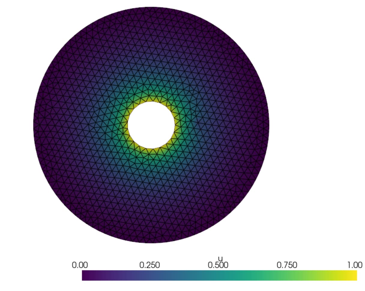
The FEniCS script that sets up and solves the above problem is given next.
from dolfin import *
from mshr import *
import math

Re = 5.
Ri = 1.

domain = Circle(Point(0., 0.), Re, 100) - Circle(Point(0., 0.), Ri, 100)
mesh = generate_mesh(domain, 40)
V = FunctionSpace(mesh, "CG", 2)
x = SpatialCoordinate(mesh)

# Define boundary subdomains
TOL = 1e-1
u_inner = Constant(1.0)
def inside(x, on_boundary):
    return near(x[0]**2 + x[1]**2, Ri**2, TOL) and on_boundary

u_outer = Constant(0.0)
def outside(x, on_boundary):
    return near(x[0]**2 + x[1]**2, Re**2, TOL) and on_boundary

inner_circ = DirichletBC(V,u_inner,inside)
outer_circ = DirichletBC(V,u_outer,outside)
bcs = [inner_circ, outer_circ]

# Defining polar coordinates
r = Expression("sqrt(x[0]*x[0]+x[1]*x[1])", degree=2)
theta = Expression("atan2(x[1],x[0])", degree=2)

# Variational formulation
u = TrialFunction(V)
v = TestFunction(V)
a1 = (u.dx(0)*v.dx(0))+(u.dx(1)*v.dx(1))
a2 = (Constant(1.0)/(r*sin(theta)))*v*(u.dx(1))
a = (a1-a2)*dx
f = Constant(0.0)
L = f*v*dx

# Compute solution
u = Function(V)
solve(a == L, u, bcs)

# writing output to file
ufile = File("sol_2d_annulus_cartesian.pvd")
ufile << u
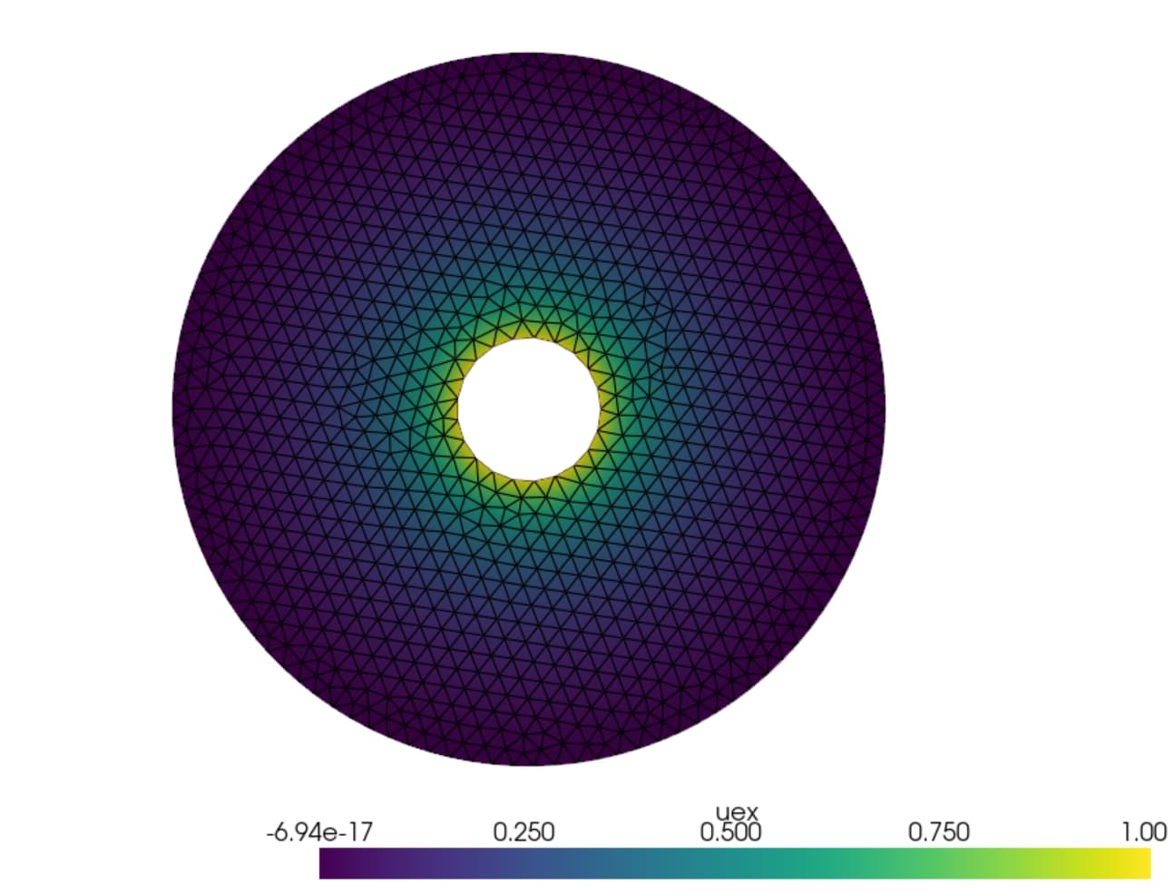
Comments and suggestions for improvement are welcome. The numerical solution may be compared against the analytical solution for the problem, which is given by
u(r)=-\left(\dfrac{R}{R-1}\right)\left[\dfrac{1}{R}-\dfrac{1}{r}\right]
Thank You
Warm Regards