Does Dolfinx's solver have an issue or require some preconditioning when handling certain meshes like the Icosahedral mesh?

I’m on modern Dolfinx version 0.10.0 running the nightly build.

The PDE being solved for is the shallow water equations

\textbf{u}_t + f(\hat{\textbf{k}}\times \textbf{u}) + g \nabla D = 0

D_t + H \nabla \cdot \textbf{u} = 0

on a spherical manifold immersed in a 3D space, where D is shallow layer depth, and \textbf{u} is the velocity, and H, g, and f are coefficients for height, gravity, and Coriolis, respectively. These two solutions can be used to yield the Kinetic and Potential energies of the system which should be conserved throughout (Total initial energy = Total final energy).

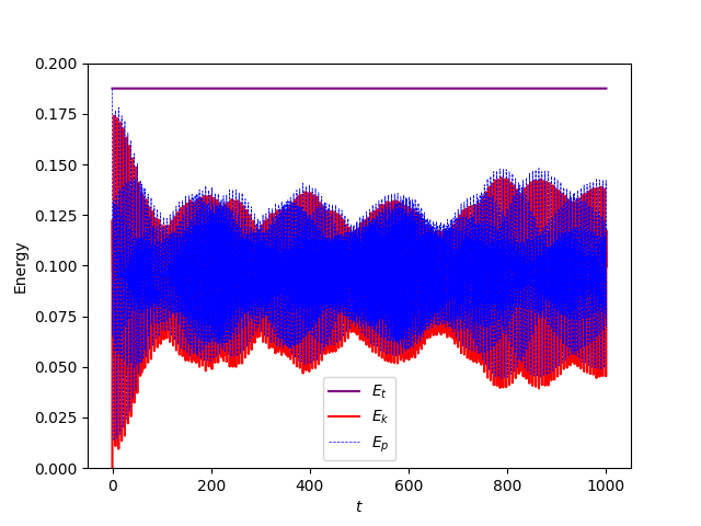
The mesh used is sphere_ico4 which can be found in this supplements file, and is an icosahedral meshed sphere, and the file solving this problem written in legacy Dolfin is linear-shallow-water.py. I attempted to adapt the code in this file to modern Dolfinx with the code below which is yielding unusual results

from mpi4py import MPI
import numpy as np
import ufl
import basix.ufl
import dolfinx as df
from petsc4py import PETSc
from dolfinx.fem import petsc

def initial_conditions(S, V):
    u0 = df.fem.Function(S)
    u0.interpolate(lambda x: np.zeros(x[:S.mesh.topology.dim].shape))
    D0 = df.fem.Function(V)
    D0.interpolate(lambda x: np.exp(-((-x[1]-1)/0.1)**2) )
    return (u0, D0)
def energy(u, D, H, g):
    kinetic = 0.5*H*ufl.dot(u,u)*ufl.dx # 0.5*H*dot(u, u)*dx
    potential = 0.5*g*D*D*ufl.dx # 0.5*g*D*D*dx
    return kinetic, potential


import meshio
tmp_data = meshio.dolfin.read("supplement/examples/mixed-poisson/hdiv-l2/meshes/sphere_ico4.xml")

mesh = df.mesh.create_mesh(
    comm=MPI.COMM_WORLD,
    cells=tmp_data.cells_dict["triangle"],
    x=tmp_data.points,
    e=ufl.Mesh(basix.ufl.element("Lagrange", "triangle", 1, shape=(3,))),
)

'''
Remove quotations to run code with custom spherical mesh

import gmsh
order = 1
res = 0.25
gmsh.initialize()
outer_sphere = gmsh.model.occ.addSphere(0, 0, 0, 1)
gmsh.model.occ.synchronize()
boundary = gmsh.model.getBoundary([(3, outer_sphere)], recursive=False)
gmsh.model.addPhysicalGroup(boundary[0][0], [boundary[0][1]], tag=1)
gmsh.option.setNumber("Mesh.CharacteristicLengthFactor", res)
gmsh.model.mesh.generate(2)
gmsh.model.mesh.setOrder(order)

mesh_data = df.io.gmshio.model_to_mesh(gmsh.model, MPI.COMM_WORLD, 0, gdim=3)

mesh = mesh_data.mesh
'''
x = ufl.SpatialCoordinate(mesh)

# mixed functionspace
S = df.fem.functionspace(mesh, ("RT", 1))
V = df.fem.functionspace(mesh, ("DG", 0))
W = ufl.MixedFunctionSpace(*(S, V))

u, D = ufl.TrialFunctions(W)
w, phi = ufl.TestFunctions(W)

# Set global orientation of test and trial vectors
global_orientation = ufl.sign(ufl.dot(x, ufl.CellNormal(mesh)))
u_ = global_orientation * u
w_ = global_orientation * w

# Setting up perp operator
k = ufl.CellNormal(mesh)

# Extract initial conditions
u_n, D_n = initial_conditions(S,V)

# Extract some parameters for discretization
dt = 0.05
f = x[2]
H = 1.0
g = 1.0

# Implicit midoint scheme discretization in time
u_mid = 0.5*(u_ + u_n)
D_mid = 0.5*(D + D_n)

# n x u_mid
u_perp = ufl.cross(k,u_mid)

# variational form
F = ufl.inner(u_ - u_n, w_)*ufl.dx 
F -= dt*ufl.div(w_)*g*D_mid*ufl.dx 
F += dt*f*ufl.inner(u_perp, w_)*ufl.dx 
F += ufl.inner(D - D_n, phi)*ufl.dx 
F += dt*H*ufl.div(u_mid)*phi*ufl.dx
a, L = ufl.system(F)

# Preassemble matrix (because we can)
A = ufl.extract_blocks(a)

# Define energy functional
kinetic_func, potential_func = energy(u_n, D_n, H, g)

# Setup solution function for current time
u_h = df.fem.Function(S)
D_h = df.fem.Function(V)

# Predefine b (for the sake of reuse of memory)
b = ufl.extract_blocks(L)

# Set-up linear solver (so that we can reuse LU)
petsc_options = {
    "ksp_type": "preonly",
    "pc_type": "lu",
    "pc_factor_mat_solver_type": "mumps",
    "ksp_error_if_not_converged": True,
}
problem = petsc.LinearProblem(
    A,
    b,
    bcs=[],
    u = [u_h,D_h],
    petsc_options=petsc_options,
    petsc_options_prefix="mixed_poisson_",
    kind="mpi",
)
u_h, D_h = problem.solve()

# Set-up some time related variables
k = 0
t = 0.0
T = 10.0

# Output initial energy
E_k = mesh.comm.allreduce(df.fem.assemble_scalar(df.fem.form(kinetic_func)), op = MPI.SUM)
E_p = mesh.comm.allreduce(df.fem.assemble_scalar(df.fem.form(potential_func)), op = MPI.SUM)
print(t, E_k, E_p, E_k + E_p, D_n.x.petsc_vec.min(), D_n.x.petsc_vec.max())
Es = np.array([[t,E_k,E_p, E_k+E_p]])

# Primers
t = 0
k = 0

# Time Loop
while(t < (T - 0.5*dt)):
    u_h, D_h = problem.solve()
    # Update u_n
    u_n.x.array[:] = u_h.x.array
    # Update D_n
    D_n.x.array[:] = D_h.x.array

    # Update time and counter
    t = np.round(t+dt,3)
    k += 1

    # Output current energy and max/min depth
    E_k = mesh.comm.allreduce(df.fem.assemble_scalar(df.fem.form(kinetic_func)), op = MPI.SUM)
    E_p = mesh.comm.allreduce(df.fem.assemble_scalar(df.fem.form(potential_func)), op = MPI.SUM)
    Es = np.vstack((Es,[t,E_k,E_p,E_k+E_p]))

t = Es[:,0]
E_k = Es[:,1]
E_p = Es[:,2]
E_t = Es[:,3]

import matplotlib.pyplot as plt

fig = plt.figure()
ax = fig.add_subplot()
ax.plot(t,E_t,label = "$E_t$", color = 'purple')
ax.plot(t,E_k,label = "$E_k$", color = 'red')
ax.plot(t,E_p,label = "$E_p$", color = 'blue', linestyle = '--', linewidth = 0.5)
ax.set_ylim(0.0,0.20)
ax.set_ylabel("Energy")
ax.set_xlabel("$t$")
ax.legend()
ax.set_title("Energies obtained using sphere_ico4")
plt.show()

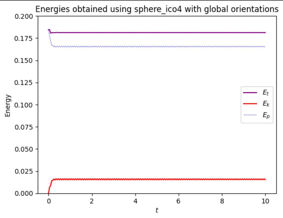
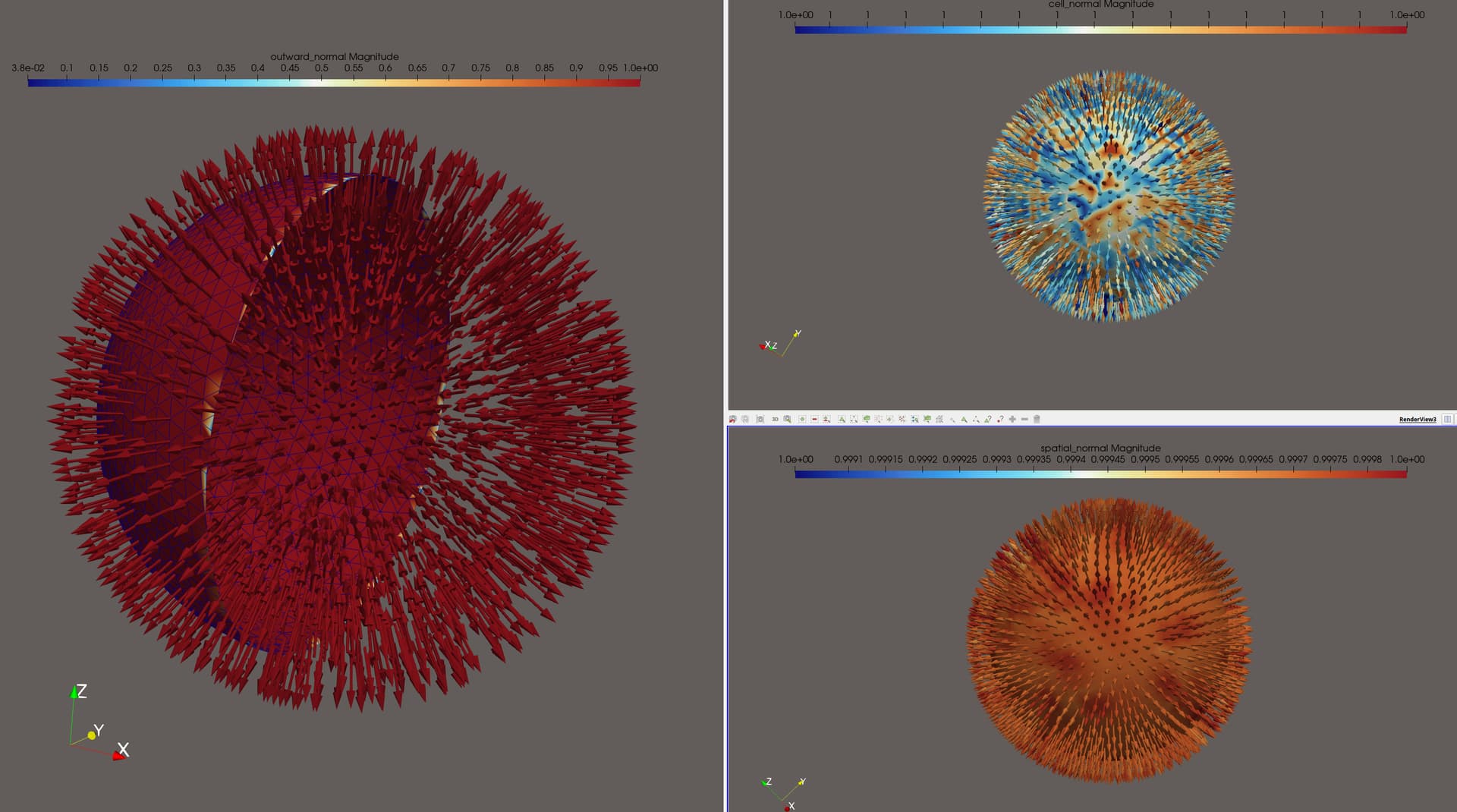
(I feel it’s important to mention that since this is a mixed problem where one of the solutions is a vector field, and we therefore opt to div-conforming space “RT”, and because of this, following this example handling a similar case (which modernizes the legacy Dolfin code in mixed-poisson-sphere.py in the same supplements file,) my code also includes global_orientation operating onto the vectors created in the RT space since (quoting Dokken here) “you have to encode the global orientation” when dealing with a RT space. That’s what this line does and why we use u_ and w_. This will also need to come back up again should I choose to plot the u_n vectors as their orientations will be off.)

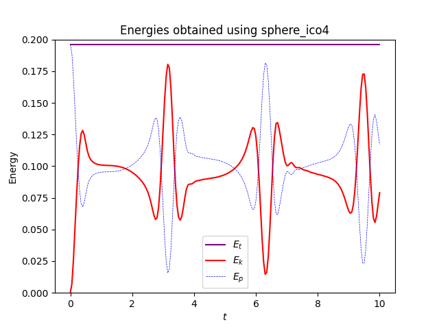
The plot should instead look exactly like this:

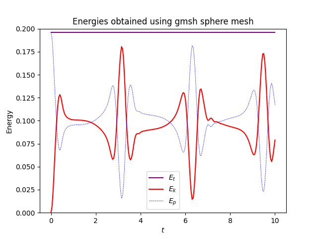
which are the results created from running the exact same code as above, but instead of the icosahdral spherical manifold, it uses a different spherical manifold which was generated in gmsh in the commented out code. I went ahead and plotted time evolutions of u and D (from an xz view) as well so see what might be happening

D_time_ico4(1)

u_time_ico4

where it looks like they move forward for a frame before getting stuck for the remainder of time.

Here are what the solutions look like using the gmsh generated mesh instead

u_time_custom(2)

D_time_custom(1)

where they both evolve with time. I find it weird that the solution appears to bounce back and forth in the gifs and the energies plot rather than evolve and spread over the entire sphere, and the only thing I’ve changed between the cases was the mesh used. This issue persists with the other icosahedral meshes in the file which are simply different resolutions of the same mesh.

The code to create the gifs

# Initialize gif

import pyvista as pv

PlottingMesh = df.fem.functionspace(mesh, ("CG", 1))
W_v = df.fem.functionspace(mesh, ("DG", 0, (mesh.geometry.dim, ))) # for vectors

pv.start_xvfb()

grid_D,grid_u = pv.UnstructuredGrid(*df.plot.vtk_mesh(PlottingMesh)),pv.UnstructuredGrid(*df.plot.vtk_mesh(PlottingMesh))

plotter = pv.Plotter()
plotter.open_gif("D_time_ico4.gif", fps=10)
grid_D["D"] = D_h.x.array
grid_D.set_active_scalars("D")

sargs = dict(title_font_size=25, label_font_size=20, fmt="%.2e", color="black",
             position_x=0.1, position_y=0.8, width=0.8, height=0.1)

renderer = plotter.add_mesh(grid_D,scalars = "D", show_edges=True, lighting=False,
                            cmap="bwr", scalar_bar_args=sargs,
                            clim=[0, max(D_h.x.array)])
plotter.view_xz()

u_d = df.fem.Function(W_v)
expr_d = df.fem.Expression(ufl.as_vector(u_h*global_orientation),W_v.element.interpolation_points)
u_d.interpolate(expr_d)
num_dofs = W_v.dofmap.index_map.size_local
num_verts = W_v.mesh.topology.index_map(0).size_local
vectors = np.zeros((num_dofs, 3), dtype=np.float64)
vectors[:, :mesh.geometry.dim] = u_d.x.array.real.reshape(num_dofs, W_v.dofmap.index_map_bs)

grid_u['vectors'] = vectors
pl = pv.Plotter()
pl.open_gif("u_time_ico4.gif", fps=10)

# Set-up some time related variables
k = 0
t = 0.0

T = 10.0

# Output initial energy
E_k = mesh.comm.allreduce(df.fem.assemble_scalar(df.fem.form(kinetic_func)), op = MPI.SUM)
E_p = mesh.comm.allreduce(df.fem.assemble_scalar(df.fem.form(potential_func)), op = MPI.SUM)
print(t, E_k, E_p, E_k + E_p, D_n.x.petsc_vec.min(), D_n.x.petsc_vec.max())
Es = np.array([[t,E_k,E_p, E_k+E_p]])

# Primers
t = 0
k = 0

# Time Loop
while(t < (T - 0.5*dt)):
    u_h, D_h = problem.solve()
    # Update u_n
    u_n.x.array[:] = u_h.x.array
    # Update D_n
    D_n.x.array[:] = D_h.x.array

    # Update plot
    
    grid_D["D"] = D_h.x.array
    plotter.write_frame()
    
    
    expr_d = df.fem.Expression(ufl.as_vector(u_h*global_orientation),W_v.element.interpolation_points)
    u_d.interpolate(expr_d)
    vectors = np.zeros((num_dofs, 3), dtype=np.float64)
    vectors[:, :mesh.geometry.dim] = u_d.x.array.real.reshape(num_dofs, W_v.dofmap.index_map_bs)
    grid_u['vectors'][:] = vectors
    glyphs = grid_u.glyph(orient='vectors', scale='vectors', factor=0.3, geom=pv.Arrow())
    pl.add_mesh(grid_u, color = "white", show_edges= True)
    pl.add_mesh(glyphs, show_scalar_bar=False, lighting=False, cmap='bwr')
    pl.view_xz()
    pl.write_frame()
    pl.clear()
    # Update time and counter
    t = np.round(t+dt,3)
    k += 1
 
    # Output current energy and max/min depth
    E_k = mesh.comm.allreduce(df.fem.assemble_scalar(df.fem.form(kinetic_func)), op = MPI.SUM)
    E_p = mesh.comm.allreduce(df.fem.assemble_scalar(df.fem.form(potential_func)), op = MPI.SUM)
    Es = np.vstack((Es,[t,E_k,E_p,E_k+E_p]))
    
pl.close()
plotter.close()

where some lines were also added to the while loop to update the plot. Take a bit over a minute to finish.

As I have stated in multiple private messages; Any field that is RT based on a manifold should be multiplied by the global orientation vector.
This includes u_n.
If you modify your code to do this, you get:

from mpi4py import MPI
import numpy as np
import ufl
from typing import Optional

import basix.ufl
import dolfinx as df
from petsc4py import PETSc
from dolfinx.fem import petsc

class Projector:
    """
    Projector for a given function.
    Solves Ax=b, where

    .. highlight:: python
    .. code-block:: python

        u, v = ufl.TrialFunction(Space), ufl.TestFunction(space)
        dx = ufl.Measure("dx", metadata=metadata)
        A = inner(u, v) * dx
        b = inner(function, v) * dx(metadata=metadata)

    Args:
        function: UFL expression of function to project
        space: Space to project function into
        petsc_options: Options to pass to PETSc
        jit_options: Options to pass to just in time compiler
        form_compiler_options: Options to pass to the form compiler
        metadata: Data to pass to the integration measure
    """

    _A: PETSc.Mat  # The mass matrix
    _b: PETSc.Vec  # The rhs vector
    _lhs: df.fem.Form  # The compiled form for the mass matrix
    _ksp: PETSc.KSP  # The PETSc solver
    _x: df.fem.Function  # The solution vector
    _dx: ufl.Measure  # Integration measure

    def __init__(
        self,
        space: df.fem.FunctionSpace,
        petsc_options: Optional[dict] = None,
        jit_options: Optional[dict] = None,
        form_compiler_options: Optional[dict] = None,
        metadata: Optional[dict] = None,
    ):
        petsc_options = {} if petsc_options is None else petsc_options
        jit_options = {} if jit_options is None else jit_options
        form_compiler_options = {} if form_compiler_options is None else form_compiler_options

        # Assemble projection matrix once
        u = ufl.TrialFunction(space)
        v = ufl.TestFunction(space)
        self._dx = ufl.Measure("dx", domain=space.mesh, metadata=metadata)
        a = ufl.inner(u, v) * self._dx(metadata=metadata)
        self._lhs = df.fem.form(a, jit_options=jit_options, form_compiler_options=form_compiler_options)
        self._A = df.fem.petsc.assemble_matrix(self._lhs)
        self._A.assemble()

        # Create vectors to store right hand side and the solution
        self._x = df.fem.Function(space)
        self._b = df.fem.Function(space)

        # Create Krylov Subspace solver
        self._ksp = PETSc.KSP().create(space.mesh.comm)
        self._ksp.setOperators(self._A)

        # Set PETSc options
        prefix = f"projector_{id(self)}"
        opts = PETSc.Options()
        opts.prefixPush(prefix)
        for k, v in petsc_options.items():
            opts[k] = v
        opts.prefixPop()
        self._ksp.setFromOptions()
        for opt in opts.getAll().keys():
            del opts[opt]

        # Set matrix and vector PETSc options
        self._A.setOptionsPrefix(prefix)
        self._A.setFromOptions()
        self._b.x.petsc_vec.setOptionsPrefix(prefix)
        self._b.x.petsc_vec.setFromOptions()

    def reassemble_lhs(self):
        df.fem.petsc.assemble_matrix(self._A, self._lhs)
        self._A.assemble()

    def assemble_rhs(self, h: ufl.core.expr.Expr):
        """
        Assemble the right hand side of the problem
        """
        v = ufl.TestFunction(self._b.function_space)
        rhs = ufl.inner(h, v) * self._dx
        rhs_compiled = df.fem.form(rhs)
        self._b.x.array[:] = 0.0
        df.fem.petsc.assemble_vector(self._b.x.petsc_vec, rhs_compiled)
        self._b.x.petsc_vec.ghostUpdate(addv=PETSc.InsertMode.ADD_VALUES, mode=PETSc.ScatterMode.REVERSE)
        self._b.x.petsc_vec.ghostUpdate(addv=PETSc.InsertMode.INSERT_VALUES, mode=PETSc.ScatterMode.FORWARD)

    def project(self, h: ufl.core.expr.Expr) -> df.fem.Function:
        """
        Compute projection using a PETSc KSP solver

        Args:
            assemble_rhs: Re-assemble RHS and re-apply boundary conditions if true
        """
        self.assemble_rhs(h)
        self._ksp.solve(self._b.x.petsc_vec, self._x.x.petsc_vec)
        return self._x

    def __del__(self):
        self._A.destroy()
        self._ksp.destroy()


def initial_conditions(S, V):
    u0 = df.fem.Function(S)
    u0.interpolate(lambda x: np.zeros(x[:S.mesh.topology.dim].shape))
    D0 = df.fem.Function(V)
    D0.interpolate(lambda x: np.exp(-((-x[1]-1)/0.1)**2) )
    return (u0, D0)
def energy(u, D, H, g):
    kinetic = 0.5*H*ufl.dot(u,u)*ufl.dx # 0.5*H*dot(u, u)*dx
    potential = 0.5*g*D*D*ufl.dx # 0.5*g*D*D*dx
    return kinetic, potential


use_gmsh = False

if use_gmsh:
    import gmsh
    order = 1
    res = 0.25
    gmsh.initialize()
    outer_sphere = gmsh.model.occ.addSphere(0, 0, 0, 1)
    gmsh.model.occ.synchronize()
    boundary = gmsh.model.getBoundary([(3, outer_sphere)], recursive=False)
    gmsh.model.addPhysicalGroup(boundary[0][0], [boundary[0][1]], tag=1)
    gmsh.option.setNumber("Mesh.CharacteristicLengthFactor", res)
    gmsh.model.mesh.generate(2)
    gmsh.model.mesh.setOrder(order)

    mesh_data = df.io.gmshio.model_to_mesh(gmsh.model, MPI.COMM_WORLD, 0, gdim=3)

    mesh = mesh_data.mesh

else:
    import meshio
    tmp_data = meshio.dolfin.read("supplement/examples/mixed-poisson/hdiv-l2/meshes/sphere_ico4.xml")

    mesh = df.mesh.create_mesh(
    comm=MPI.COMM_WORLD,
    cells=tmp_data.cells_dict["triangle"],
    x=tmp_data.points,
    e=ufl.Mesh(basix.ufl.element("Lagrange", "triangle", 1, shape=(3,))),
)


x = ufl.SpatialCoordinate(mesh)

# mixed functionspace
S = df.fem.functionspace(mesh, ("RT", 1))
V = df.fem.functionspace(mesh, ("DG", 0))
W = ufl.MixedFunctionSpace(*(S, V))

u, D = ufl.TrialFunctions(W)
w, phi = ufl.TestFunctions(W)

# Set global orientation of test and trial vectors
global_orientation = ufl.sign(ufl.dot(x, ufl.CellNormal(mesh)))
u_ = global_orientation * u
w_ = global_orientation * w

# Setting up perp operator
k = ufl.CellNormal(mesh)

# Extract initial conditions
u_n, D_n = initial_conditions(S,V)
u_n_ = global_orientation * u_n
# Extract some parameters for discretization
dt = 0.05
f = x[2]
H = 1.0
g = 1.0

# Implicit midoint scheme discretization in time
u_mid = 0.5*(u_ + u_n_)
D_mid = 0.5*(D + D_n)

# n x u_mid
u_perp = ufl.cross(k,u_mid)

# variational form
F = ufl.inner(u_ - u_n_, w_)*ufl.dx 
F -= dt*ufl.div(w_)*g*D_mid*ufl.dx 
F += dt*f*ufl.inner(u_perp, w_)*ufl.dx 
F += ufl.inner(D - D_n, phi)*ufl.dx 
F += dt*H*ufl.div(u_mid)*phi*ufl.dx
a, L = ufl.system(F)

# Preassemble matrix (because we can)
A = ufl.extract_blocks(a)

# Define energy functional
kinetic_func, potential_func = energy(u_n, D_n, H, g)

# Setup solution function for current time
u_h = df.fem.Function(S)
D_h = df.fem.Function(V)

# Predefine b (for the sake of reuse of memory)
b = ufl.extract_blocks(L)

# Set-up linear solver (so that we can reuse LU)
petsc_options = {
    "ksp_type": "preonly",
    "pc_type": "lu",
    "pc_factor_mat_solver_type": "mumps",
    "ksp_error_if_not_converged": True,
    "ksp_monitor": None
}
problem = petsc.LinearProblem(
    A,
    b,
    bcs=[],
    u = [u_h,D_h],
    petsc_options=petsc_options,
    petsc_options_prefix="mixed_poisson_",
    kind="mpi",
)
u_h, D_h = problem.solve()

# Set-up some time related variables
k = 0
t = 0.0
T = 10.0

# Output initial energy
E_k = mesh.comm.allreduce(df.fem.assemble_scalar(df.fem.form(kinetic_func)), op = MPI.SUM)
E_p = mesh.comm.allreduce(df.fem.assemble_scalar(df.fem.form(potential_func)), op = MPI.SUM)
print(t, E_k, E_p, E_k + E_p, D_n.x.petsc_vec.min(), D_n.x.petsc_vec.max())
Es = np.array([[t,E_k,E_p, E_k+E_p]])

# Primers
t = 0
k = 0

# Time Loop
while(t < (T - 0.5*dt)):
    u_h, D_h = problem.solve()
    # Update u_n
    u_n.x.array[:] = u_h.x.array
    # Update D_n
    D_n.x.array[:] = D_h.x.array

    # Update time and counter
    t = np.round(t+dt,3)
    k += 1

    # Output current energy and max/min depth
    E_k = mesh.comm.allreduce(df.fem.assemble_scalar(df.fem.form(kinetic_func)), op = MPI.SUM)
    E_p = mesh.comm.allreduce(df.fem.assemble_scalar(df.fem.form(potential_func)), op = MPI.SUM)
    Es = np.vstack((Es,[t,E_k,E_p,E_k+E_p]))

V_out = df.fem.functionspace(mesh, ("DG", 2, (mesh.geometry.dim, )))
projector = Projector(V_out, {"ksp_error_if_not_converged": True, "ksp_typ": "preonly",
                              "pc_type": "lu", "pc_factor_mat_solver_type":"mumps"})
_x = projector.project(global_orientation*u_h)

with df.io.VTXWriter(mesh.comm, f"u_h{use_gmsh}.bp", [_x]) as bp:
    bp.write(0.0)

t = Es[:,0]
E_k = Es[:,1]
E_p = Es[:,2]
E_t = Es[:,3]

import matplotlib.pyplot as plt

fig = plt.figure()
ax = fig.add_subplot()
ax.plot(t,E_t,label = "$E_t$", color = 'purple')
ax.plot(t,E_k,label = "$E_k$", color = 'red')
ax.plot(t,E_p,label = "$E_p$", color = 'blue', linestyle = '--', linewidth = 0.5)
ax.set_ylim(0.0,0.20)
ax.set_ylabel("Energy")
ax.set_xlabel("$t$")
ax.legend()
if use_gmsh:
    ax.set_title("Energies obtained using gmsh sphere mesh")
else:
    ax.set_title("Energies obtained using sphere_ico4")
plt.savefig(f"energy_gmsh_{use_gmsh}.png")

which in turn outputs


1 Like

And now the gif plots are working properly as well

u_time_ico4

D_time_ico4

and it looks like the waves now propagate symmetrically, whereas for the gmsh mesh, the waves end up being asymmetric. So it wasn’t an issue with the mesh, but my oversight in applying the orientation to the initial condition because I failed to realize that initial vector is also a vector created in the RT function space.

It’s weird that energies for the 2 different meshes are different though. Out of curiosity, I decided to plot the evolution of the energies of the system over 1000 seconds to see how they compared

and the differences are now more pronounced. Could that be an issue isolated to the mesh used?

This kind of problem, when using a linear grid, not quadratic, will of course show mesh dependence. Under refinement (that respects the curvature of the original sphere) these should converge

1 Like

I’m sorry, I had the plots switched. This plot uses the icosahedral mesh, sphere_ico4

and here is the one obtained using the gmsh mesh for comparison

Additionally, I found out that my first icosahedral plot over 1000 seconds used sphere_ico5, which is a higher resolution version of sphere_ico4 (and sphere_ico6 is a higher resolution version of sphere_ico5, they all seem to use the same base sphere and increase resolution as the number in the name increases). If I compare the results for the 2 different resolutions of the same icosahedral style mesh, the results are visibly indistinguishable, so resolution is not the culprit in causing the icosphere mesh’s results not converging to those in the paper.

I looked it up, and yes, it is the case that legacy Dolfin .xml meshes only supported up to first order, or linear meshes. Setting the div conforming functionspace created from this first degree icosahedral mesh to 2nd degree, or quadratic (and the corresponding scalar space to degree-1), by running

S = df.fem.functionspace(mesh, ("RT", 2))
V = df.fem.functionspace(mesh, ("DG", 1))
W = ufl.MixedFunctionSpace(*(S, V))

changed the results to

This plot shows that the energies are now closer to those shown in the paper, but are not exact. Here is the 1000 second plot, in case you were curious

If what you instead meant was modifying the mesh itself to make it second order, I haven’t figured out how to do that. I did find this post which talked about it, but it’s possibly outdated due to being about 6 years old and over 200 messages long. Here’s what I tried:

import meshio
import gmsh

meshfile = "supplement/examples/mixed-poisson/hdiv-l2/meshes/sphere_ico4.xml"
mesh = meshio.read(meshfile)
meshio.write("sphere_ico4.xdmf", mesh)
gmsh.initialize()
gmsh.open("sphere_ico4.xdmf")
gmsh.model.mesh.setOrder(2)

but I wasn’t able to open the converted .xdmf file due to an error

Error   : 'sphere_ico4.xdmf', line 0: syntax error (<)

---------------------------------------------------------------------------
Exception                                 Traceback (most recent call last)
/tmp/ipykernel_1832/3453081995.py in ?()
----> 1 gmsh.open("sphere_ico4.xdmf")
      2 gmsh.model.mesh.setOrder(2)

/usr/local/lib/gmsh.py in ?(fileName)
    342     lib.gmshOpen(
    343         c_char_p(fileName.encode()),
    344         byref(ierr))
    345     if ierr.value != 0:
--> 346         raise Exception(logger.getLastError())

Exception: 'sphere_ico4.xdmf', line 0: syntax error (<)

So, if that’s what you meant for me to do, I haven’t figured out how to do that yet.

Dear Fea,

A few things here:

  1. The paper specifies:

    while f in your code is x[2], which will yield different results.
  2. The OutwardNormal function that is used in the inner product in the original paper seem rather strange to me, as it is mesh dependent. You can verify this by switching it with a normalized outwards pointing normal, which will then yield (unsymmetric) results for the wave profile, similar to what happens in DOLFINx if you use the globally oriented CellNormal (i.e. multiplied by global orientation).

There are too many minuses here to match the initial condition in the original code.

  1. Different meshes (especially that resolves the curvature of the sphere differently, will yield different results.
  2. If you instead of comparing with the paper, run the code supplied by Marie (which I below has slightly adapted to make it work with legacy DOLFIN master branch, you get:
"""
Linear shallow water code for mimetic element pairs.

The equations are the linear shallow water equations.  Let u be
velocity, D be depth _perturbation_, g = gravity, H = base layer depth

du/dt + fu^\perp = -g grad(D)
dD/dt + H div(u) = 0

In the continuous case, if we pick a velocity field u = curl(psi),
then div(u) = 0, so dD/dt is initially 0.  If you then choose D to
satisfy fu^\perp = -g grad(D), du/dt is initially 0 also.  Then both u
and D remain fixed for all time.  This is known as "geostrophic
balance".  One of the special properties of the spatial discretisation
is that it represents this balance.

With implicit midpoint timestepping, the scheme conserves energy -
this is verified in.
"""

# Copyright (C) 2013 Andrew McRae and Imperial College London
# Written by Andrew McRae and Colin J. Cotter
# Modified by Marie E. Rognes (meg@simula.no), 2013
# Modified by Jørgen S. Dokken (dokken@simula.no), 2025

from dolfin import *

parameters["form_compiler"]["cpp_optimize"] = True
parameters["form_compiler"]["optimize"] = True


class OutwardNormal(UserExpression):
    def __init__(self, mesh, *arg, **kwargs):
        super().__init__(*arg, **kwargs)
        self.mesh = mesh

    def eval_cell(self, values, x, cell):
        c = Cell(self.mesh, cell.index)
        normal = c.cell_normal()
        scale = 1 if c.orientation == 0 else -1
        values[0] = normal[0] * scale
        values[1] = normal[1] * scale
        values[2] = normal[2] * scale

    def value_shape(self):
        return (3,)


def initialize_parameters(verbose=True):
    # Create application parameters
    params = Parameters("Discretization")
    params.add("family", "RT")
    params.add("order", 1)
    params.add("meshid", "sphere_ico4")
    params.add("store_pvds", True)
    params.add("T", 10.0)
    params.add("dt", 0.05)
    params.add("directory", "default")

    # Read parameters from the command-line
    params.parse()
    if params["directory"] == "default":
        default = "%s%d_%s" % (params["family"], params["order"], params["meshid"])
        params["directory"] = default

    info(params, verbose)

    # Return parameters
    return params


def create_function_spaces(mesh, family, order):
    s_el = FiniteElement(family, mesh.ufl_cell(), order)
    v_el = FiniteElement("DG", mesh.ufl_cell(), order - 1)
    me = MixedElement([s_el, v_el])
    W = FunctionSpace(mesh, me)
    PlottingMesh = VectorFunctionSpace(mesh, "CG", order)
    return (W, PlottingMesh)


def myperp(u):
    return cross(en_exp, u)


def initial_conditions(W):
    w_ = Function(W)
    w_.vector()[:] = 0.0
    W1 = W.sub(1).collapse()

    w1 = project(Expression("exp(-pow((-x[1]-1.0)/0.1, 2))", degree=2), W1)
    fa = FunctionAssigner(W.sub(1), W1)
    fa.assign(
        w_.sub(1),
        w1,
    )
    return w_


def energy(u, D, H, g):
    kinetic = 0.5 * H * dot(u, u) * dx
    potential = 0.5 * g * D * D * dx
    return (kinetic, potential)


def output_energy(energyfile, t, kinetic, potential):
    energyfile.write("times.append(%g);\n" % t)
    energyfile.write("kinetics.append(%.18g);\n" % kinetic)
    energyfile.write("potentials.append(%.18g);\n" % potential)


def main():
    # Setup parameters
    params = initialize_parameters()

    # Store parameters
    storage = "results/%s" % params["directory"]
    paramsfile = File("%s/application_parameters.xml" % storage)
    paramsfile << params

    # Set-up storage for energies
    energyfilename = "results/%s/energies.py" % params["directory"]
    print(("Storing energies to %s" % energyfilename))
    energyfile = open(energyfilename, "w")
    energyfile.write("# Results from linear shallow water test case.\n")
    energyfile.write("kinetics = [];\n")
    energyfile.write("potentials = [];\n")
    energyfile.write("times = [];\n")

    # Initialize mesh
    mesh = Mesh("../mixed-poisson/hdiv-l2/meshes/%s.xml.gz" % params["meshid"])
    global_normal = Expression(("x[0]", "x[1]", "x[2]"), degree=1)
    mesh.init_cell_orientations(global_normal)

    # Set-up function spaces
    (W, PlottingMesh) = create_function_spaces(mesh, params["family"], params["order"])

    # Setting up perp operator
    outward_normals = OutwardNormal(mesh)

    perp = lambda u: cross(outward_normals, u)

    # Extract initial conditions
    w_ = initial_conditions(W)
    (u_, D_) = split(w_)
    # Extract some parameters for discretization
    dt = Constant(params["dt"])
    f = Expression("x[2]", degree=1)
    H = 1.0
    g = 1.0

    # Implicit midoint scheme discretization in time
    (u, D) = TrialFunctions(W)
    (w, phi) = TestFunctions(W)
    u_mid = 0.5 * (u + u_)
    D_mid = 0.5 * (D + D_)
    F = (
        inner(u - u_, w)
        - dt * div(w) * g * D_mid
        + dt * f * inner(perp(u_mid), w)
        + inner(D - D_, phi)
        + dt * H * div(u_mid) * phi
    ) * dx
    (a, L) = system(F)

    # Preassemble matrix (because we can)
    A = assemble(a)

    # Define energy functional
    (kinetic_func, potential_func) = energy(u_, D_, H, g)

    # Setup solution function for current time
    uD = Function(W)

    # Predefine b (for the sake of reuse of memory)
    b = Function(W).vector()

    # Set-up linear solver (so that we can reuse LU)
    solver = LUSolver(A)

    # Set-up some pvd storage
    if params["store_pvds"]:
        ufile = File("%s/pvds/u.pvd" % storage)
        Dfile = File("%s/pvds/D.pvd" % storage)

    # Set-up some time related variables
    k = 0
    t = 0.0
    T = params["T"]
    dt = float(dt)

    # Output initial energy
    E_k = assemble(kinetic_func)
    E_p = assemble(potential_func)
    print(
        t,
        E_k,
        E_p,
        E_k + E_p,
        w_.sub(1, deepcopy=True).vector().min(),
        w_.sub(1, deepcopy=True).vector().max(),
    )
    output_energy(energyfile, t, E_k, E_p)

    # Time loop
    while t < (T - 0.5 * dt):
        # Assemble right-hand side, reuse b
        assemble(L, tensor=b)

        # Solve system
        solver.solve(uD.vector(), b)

        # Update previous solution
        u, D = uD.split()
        w_.assign(uD)

        # Update time and counter
        t += dt
        k += 1

        # Output current energy and max/min depth
        E_k = assemble(kinetic_func)
        E_p = assemble(potential_func)
        print(
            t,
            E_k,
            E_p,
            E_k + E_p,
            w_.sub(1, deepcopy=True).vector().min(),
            w_.sub(1, deepcopy=True).vector().max(),
        )
        output_energy(energyfile, t, E_k, E_p)

        # Store solutions to xml and pvd
        solutionfile = File("%s/xmls/uD_%d.xml.gz" % (storage, k))
        solutionfile << uD

        if params["store_pvds"]:
            uplot = project(u, PlottingMesh)
            ufile << uplot
            Dfile << D


if __name__ == "__main__":
    main()

with the plotting script:

"""
Plotting script for energies based on precomputed values
"""

# Copyright (C) 2013 Marie E. Rognes

import os
import sys
import pylab
import numpy

if len(sys.argv) < 2:
    print("Usage: python plot_energies.py results-directory")
    sys.exit()

resultsdir = sys.argv[1]
resultspath = os.path.join(os.getcwd(), resultsdir)
print("Treating data from %s" % resultspath)
sys.path.insert(0, resultspath)

# Increase fonts
myfontsize = 26
# pylab.rc("lines", linewidth=2)
# pylab.rc("legend", fontsize=0.8 * myfontsize)
# pylab.rc("text", fontsize=0.8 * myfontsize)
# pylab.rc("lines", markeredgewidth=2.0)

pylab.figure(figsize=(10, 8))

# Import each of the cases here
from energies import times, kinetics, potentials

pylab.plot(times, kinetics, label="$E_k$")
pylab.plot(times, potentials, label="$E_p$")
pylab.plot(times, numpy.array(kinetics) + numpy.array(potentials), label="$E_T$")

pylab.xlabel("$t$", fontsize=myfontsize)
pylab.ylabel("Energy", fontsize=myfontsize)
pylab.legend(loc="best")
pylab.grid(True)
print("Storing plot to '%s/energies.pdf'" % resultsdir)
pylab.savefig("%s/energies.pdf" % resultsdir)

print(
    "The maximum energy conservation error is %.18g"
    % max(
        abs(
            numpy.array(kinetics)
            + numpy.array(potentials)
            - (kinetics[0] + potentials[0])
        )
    )
)

pylab.savefig("test.png")

yielding


which is very similar to what I get with the DOLFINx code with the same grid and temporal discretization

If i instead run this with ico6 meshes, i get:
Legacy:

DOLFINx

GMSH grids

I would suggest that you in the above code change the outward-normal to a consistent normal vector, as I do not understand why one would have a normal vector in the variational form that is dependent on the initial orientation of the mesh. Maybe Marie can comment on this.

Higher order meshes

On manifolds, it is highly beneficial to use curved cells. These are not supported in legacy fenics, but in DOLFINx.

1 Like

I just finished converting the original xml mesh to a quadratic order equivalent of the original (I had to open the .msh file created using meshio using the gmsh GUI and export it first, then I could finally open that exported file using gmsh.open), and I got the exact same results as prior when I simply set the div conforming space to second order. So, for future reference, I’ll know to do that instead of picking apart the mesh.

Now to your reply,

That is section 5.3 which covers a special case of that in 5.2 (the case I’m working on) where f=0, and the code for this example is in the torus file. At the end of Section 5.2, it explains that figures 9 and 10 are the results obtained for the nonzero case, and the code for this example are located in the linear-shallow-water file. They both use a linear_shallow_water.py file, so that might have been confusing. Oddly enough, upon observing the files in my torus file, I notice that f is set to x[2] in that file as well, however, to simulate f being 0 in that file, they simply removed this integral dt*f*inner(perp(u_mid), w) from the variational form.

The original expression was D0 = project(Expression("exp(-pow((-x[1]-1.0)/0.1, 2))"), V), so

e^{-\big(\frac{-y-1}{0.1}\big)^2}

so np.exp(-((-x[1]-1)/0.1)**2) should translate to that; np.exp(-((x[1]+1)/0.1)**2) should also work.

Unfortunately, I do not have legacy Dolfin on my system, nor do I have any experience with it, so I’ll just have to take your word for it rather than test it for myself.

By “wave profile”, are you talking about the shallow water waves propagating outward in the gifs, or the wavy shaped energy profile that could be perceived as a sort of wave profile? In the case of the former, when using Dolfinx code which used the global normal to enforce orientation as before, the icosphere mesh produced symmetrically propagating waves, whereas the gmsh mesh produced asymmetrical ones. In the case of the latter, I think “symmetry” would refer to the symmetry about the packet of 3 crest trough couplings that occur about every 3 seconds. If that’s the case then, you bring up a concept that I found rather interesting as I moved my function space to 3rd order and higher in my Dolfinx code which used the global normal and the icosphere mesh. When the order went to 3rd order and higher, the symmetry of the individual wave packets became almost perfect. If you go into the Dolfinx code and set the functionspace to 3rd order, you can see that in the results.

Got it!

I do not have legacy Dolfin, but it is reassuring to see the results produced using their same mesh and their same code yielded the same results as ours in Dolfinx using the global normal. I would not know how to create a consistent outward normal vector in legacy Dolfin or how to enforce it, unfortunately I have never used legacy Dolfin. If you did this, did you get a different result?

I’d also be interested to hear from the author of the paper too if they’re on here.

For an example that I planned to work on after resolving this, the example deals with a geophysical fluid plotted using Earth as the sphere, so it will be important to note that my results will be highly benefited if the cells which compose my mesh are curved. That is accomplished by simply making them quadratic or higher order than linear, yes?

I am going to try to illustrate the mistake I mean exists in the legacy code with a small example:

from dolfin import *


class OutwardNormal(UserExpression):
    def __init__(self, mesh, *arg, **kwargs):
        super().__init__(*arg, **kwargs)
        self.mesh = mesh

    def eval_cell(self, values, x, cell):
        c = Cell(self.mesh, cell.index)
        normal = c.cell_normal()
        scale = 1 if c.orientation == 0 else -1
        values[0] = normal[0] * scale
        values[1] = normal[1] * scale
        values[2] = normal[2] * scale

    def value_shape(self):
        return (3,)


use_gmsh = False

if use_gmsh:
    import meshio
    import gmsh

    order = 1
    res = 0.25
    gmsh.initialize()
    outer_sphere = gmsh.model.occ.addSphere(0, 0, 0, 1)
    gmsh.model.occ.synchronize()
    boundary = gmsh.model.getBoundary([(3, outer_sphere)], recursive=False)
    gmsh.model.addPhysicalGroup(boundary[0][0], [boundary[0][1]], tag=1)
    gmsh.option.setNumber("Mesh.CharacteristicLengthFactor", res)
    gmsh.model.mesh.generate(2)
    gmsh.model.mesh.setOrder(order)
    gmsh.write("gmsh_sphere.msh")
    in_mesh = meshio.read("gmsh_sphere.msh")
    meshio.write("gmsh_sphere.xdmf", in_mesh)
    mesh = Mesh()
    with XDMFFile("gmsh_sphere.xdmf") as f:
        f.read(mesh)
else:
    mesh = Mesh("../mixed-poisson/hdiv-l2/meshes/sphere_ico4.xml")
global_normal = Expression(("x[0]", "x[1]", "x[2]"), degree=1)
mesh.init_cell_orientations(global_normal)

n = OutwardNormal(mesh)

c_n = CellNormal(mesh)

x = SpatialCoordinate(mesh)

n_x = x / sqrt(dot(x, x))


class Projector:
    def __init__(self, V):
        u = TrialFunction(V)
        v = TestFunction(V)
        a = inner(u, v) * dx
        self.A = assemble(a)
        self.solver = LUSolver(self.A)
        self.V = V

    def __call__(self, f):
        v = TestFunction(self.V)
        b = assemble(inner(f, v) * dx)
        u = Function(self.V)
        self.solver.solve(u.vector(), b)
        return u


Q = VectorFunctionSpace(mesh, "DG", 0)

projector = Projector(Q)

outward_n = projector(n)
cell_normal = projector(c_n)
spatial_normal = projector(n_x)


outward_n.rename("outward_normal", "outward_normal")
cell_normal.rename("cell_normal", "cell_normal")
spatial_normal.rename("spatial_normal", "spatial_normal")

with XDMFFile("normals.xdmf") as f:
    f.write(outward_n, 0)
    f.write(cell_normal, 0)
    f.write(spatial_normal, 0)

One can inspect all these normals in Paraview.
Using the mesh from the paper, I get:


Note that here, the “outward” normal is the only one that flips signs every now and then.
Next, if we use the gmsh mesh, we get:

where you see the exact same, fluctuating behavior in the “OutwardNormal”.

This means that it is very unclear to me how OutwardNormal should emulate the k from the paper, which is stated as:

Thus, when you look at the DOLFINx code, one should use an outward oriented normal, i.e.

k = global_orientation * ufl.CellNormal(mesh)

instead of ufl.CellNormal(mesh),
one gets very the exact same results for the old meshes and gmsh:


Full script is available below:

"""Linear shallow water equation on a manifold

Author: Jørgen S. Dokken
"""

from mpi4py import MPI
import numpy as np
import ufl
from typing import Optional

import basix.ufl
import dolfinx as df
from petsc4py import PETSc
from dolfinx.fem import petsc


class Projector:
    """
    Projector for a given function.
    Solves Ax=b, where

    .. highlight:: python
    .. code-block:: python

        u, v = ufl.TrialFunction(Space), ufl.TestFunction(space)
        dx = ufl.Measure("dx", metadata=metadata)
        A = inner(u, v) * dx
        b = inner(function, v) * dx(metadata=metadata)

    Args:
        function: UFL expression of function to project
        space: Space to project function into
        petsc_options: Options to pass to PETSc
        jit_options: Options to pass to just in time compiler
        form_compiler_options: Options to pass to the form compiler
        metadata: Data to pass to the integration measure
    """

    _A: PETSc.Mat  # The mass matrix
    _b: PETSc.Vec  # The rhs vector
    _lhs: df.fem.Form  # The compiled form for the mass matrix
    _ksp: PETSc.KSP  # The PETSc solver
    _x: df.fem.Function  # The solution vector
    _dx: ufl.Measure  # Integration measure

    def __init__(
        self,
        space: df.fem.FunctionSpace,
        petsc_options: Optional[dict] = None,
        jit_options: Optional[dict] = None,
        form_compiler_options: Optional[dict] = None,
        metadata: Optional[dict] = None,
    ):
        petsc_options = {} if petsc_options is None else petsc_options
        jit_options = {} if jit_options is None else jit_options
        form_compiler_options = (
            {} if form_compiler_options is None else form_compiler_options
        )

        # Assemble projection matrix once
        u = ufl.TrialFunction(space)
        v = ufl.TestFunction(space)
        self._dx = ufl.Measure("dx", domain=space.mesh, metadata=metadata)
        a = ufl.inner(u, v) * self._dx(metadata=metadata)
        self._lhs = df.fem.form(
            a, jit_options=jit_options, form_compiler_options=form_compiler_options
        )
        self._A = df.fem.petsc.assemble_matrix(self._lhs)
        self._A.assemble()

        # Create vectors to store right hand side and the solution
        self._x = df.fem.Function(space)
        self._b = df.fem.Function(space)

        # Create Krylov Subspace solver
        self._ksp = PETSc.KSP().create(space.mesh.comm)
        self._ksp.setOperators(self._A)

        # Set PETSc options
        prefix = f"projector_{id(self)}"
        opts = PETSc.Options()
        opts.prefixPush(prefix)
        for k, v in petsc_options.items():
            opts[k] = v
        opts.prefixPop()
        self._ksp.setFromOptions()
        for opt in opts.getAll().keys():
            del opts[opt]

        # Set matrix and vector PETSc options
        self._A.setOptionsPrefix(prefix)
        self._A.setFromOptions()
        self._b.x.petsc_vec.setOptionsPrefix(prefix)
        self._b.x.petsc_vec.setFromOptions()

    def reassemble_lhs(self):
        df.fem.petsc.assemble_matrix(self._A, self._lhs)
        self._A.assemble()

    def assemble_rhs(self, h: ufl.core.expr.Expr):
        """
        Assemble the right hand side of the problem
        """
        v = ufl.TestFunction(self._b.function_space)
        rhs = ufl.inner(h, v) * self._dx
        rhs_compiled = df.fem.form(rhs)
        self._b.x.array[:] = 0.0
        df.fem.petsc.assemble_vector(self._b.x.petsc_vec, rhs_compiled)
        self._b.x.petsc_vec.ghostUpdate(
            addv=PETSc.InsertMode.ADD_VALUES, mode=PETSc.ScatterMode.REVERSE
        )
        self._b.x.petsc_vec.ghostUpdate(
            addv=PETSc.InsertMode.INSERT_VALUES, mode=PETSc.ScatterMode.FORWARD
        )

    def project(self, h: ufl.core.expr.Expr) -> df.fem.Function:
        """
        Compute projection using a PETSc KSP solver

        Args:
            assemble_rhs: Re-assemble RHS and re-apply boundary conditions if true
        """
        self.assemble_rhs(h)
        self._ksp.solve(self._b.x.petsc_vec, self._x.x.petsc_vec)
        return self._x

    def __del__(self):
        self._A.destroy()
        self._ksp.destroy()


def initial_conditions(S, V):
    u0 = df.fem.Function(S)
    u0.interpolate(lambda x: np.zeros(x[: S.mesh.topology.dim].shape))
    D0 = df.fem.Function(V)
    D0.interpolate(lambda x: np.exp(-(((-x[1] - 1) / 0.1) ** 2)))
    return (u0, D0)


def energy(u, D, H, g):
    kinetic = 0.5 * H * ufl.dot(u, u) * ufl.dx  # 0.5*H*dot(u, u)*dx
    potential = 0.5 * g * D * D * ufl.dx  # 0.5*g*D*D*dx
    return kinetic, potential


use_gmsh = True

if use_gmsh:
    import gmsh

    order = 1
    res = 0.1
    gmsh.initialize()
    outer_sphere = gmsh.model.occ.addSphere(0, 0, 0, 1)
    gmsh.model.occ.synchronize()
    boundary = gmsh.model.getBoundary([(3, outer_sphere)], recursive=False)
    gmsh.model.addPhysicalGroup(boundary[0][0], [boundary[0][1]], tag=1)
    gmsh.option.setNumber("Mesh.CharacteristicLengthFactor", res)
    gmsh.model.mesh.generate(2)
    gmsh.model.mesh.setOrder(order)

    mesh_data = df.io.gmshio.model_to_mesh(gmsh.model, MPI.COMM_WORLD, 0, gdim=3)

    mesh = mesh_data.mesh

else:
    import meshio

    tmp_data = meshio.dolfin.read(
        "../../examples/mixed-poisson/hdiv-l2/meshes/sphere_ico6.xml"
    )

    mesh = df.mesh.create_mesh(
        comm=MPI.COMM_WORLD,
        cells=tmp_data.cells_dict["triangle"],
        x=tmp_data.points,
        e=ufl.Mesh(basix.ufl.element("Lagrange", "triangle", 1, shape=(3,))),
    )


x = ufl.SpatialCoordinate(mesh)

# mixed functionspace
S = df.fem.functionspace(mesh, ("RT", 1))
V = df.fem.functionspace(mesh, ("DG", 0))
W = ufl.MixedFunctionSpace(*(S, V))

u, D = ufl.TrialFunctions(W)
w, phi = ufl.TestFunctions(W)

# Set global orientation of test and trial vectors
global_orientation = ufl.sign(ufl.dot(x, ufl.CellNormal(mesh)))
u_ = global_orientation * u
w_ = global_orientation * w

# Setting up perp operator
k = global_orientation * ufl.CellNormal(mesh)

# Extract initial conditions
u_n, D_n = initial_conditions(S, V)
u_n_ = global_orientation * u_n
# Extract some parameters for discretization
dt = 0.05
f = x[2]
H = 1.0
g = 1.0

# Implicit midoint scheme discretization in time
u_mid = 0.5 * (u_ + u_n_)
D_mid = 0.5 * (D + D_n)

# n x u_mid
u_perp = ufl.cross(k, u_mid)

# variational form
F = ufl.inner(u_ - u_n_, w_) * ufl.dx
F -= dt * ufl.div(w_) * g * D_mid * ufl.dx
F += dt * f * ufl.inner(u_perp, w_) * ufl.dx
F += ufl.inner(D - D_n, phi) * ufl.dx
F += dt * H * ufl.div(u_mid) * phi * ufl.dx
a, L = ufl.system(F)

# Preassemble matrix (because we can)
A = ufl.extract_blocks(a)

# Define energy functional
kinetic_func, potential_func = energy(u_n, D_n, H, g)

# Setup solution function for current time
u_h = df.fem.Function(S)
D_h = df.fem.Function(V)

# Predefine b (for the sake of reuse of memory)
b = ufl.extract_blocks(L)

# Set-up linear solver (so that we can reuse LU)
petsc_options = {
    "ksp_type": "preonly",
    "pc_type": "lu",
    "pc_factor_mat_solver_type": "mumps",
    "ksp_error_if_not_converged": True,
    "ksp_monitor": None,
}
problem = petsc.LinearProblem(
    A,
    b,
    bcs=[],
    u=[u_h, D_h],
    petsc_options=petsc_options,
    petsc_options_prefix="mixed_poisson_",
    kind="mpi",
)
u_h, D_h = problem.solve()

# Set-up some time related variables
k = 0
t = 0.0
T = 10.0

# Output initial energy
E_k = mesh.comm.allreduce(df.fem.assemble_scalar(df.fem.form(kinetic_func)), op=MPI.SUM)
E_p = mesh.comm.allreduce(
    df.fem.assemble_scalar(df.fem.form(potential_func)), op=MPI.SUM
)
print(t, E_k, E_p, E_k + E_p, D_n.x.petsc_vec.min(), D_n.x.petsc_vec.max())
Es = np.array([[t, E_k, E_p, E_k + E_p]])

# Primers
t = 0
k = 0
V_out = df.fem.functionspace(mesh, ("DG", 2, (mesh.geometry.dim,)))
projector = Projector(
    V_out,
    {
        "ksp_error_if_not_converged": True,
        "ksp_typ": "preonly",
        "pc_type": "lu",
        "pc_factor_mat_solver_type": "mumps",
    },
)
_x = projector.project(global_orientation * u_h)
_x.name = f"u_use_gmsh={use_gmsh}"
vtx = df.io.VTXWriter(mesh.comm, f"u_h{use_gmsh}.bp", [_x])


# Time Loop
while t < (T - 0.5 * dt):
    u_h, D_h = problem.solve()
    # Update u_n
    u_n.x.array[:] = u_h.x.array
    # Update D_n
    D_n.x.array[:] = D_h.x.array

    # Update time and counter
    t = np.round(t + dt, 3)
    k += 1

    # Output current energy and max/min depth
    E_k = mesh.comm.allreduce(
        df.fem.assemble_scalar(df.fem.form(kinetic_func)), op=MPI.SUM
    )
    E_p = mesh.comm.allreduce(
        df.fem.assemble_scalar(df.fem.form(potential_func)), op=MPI.SUM
    )
    Es = np.vstack((Es, [t, E_k, E_p, E_k + E_p]))
    _x = projector.project(global_orientation * u_h)
    vtx.write(t)


t = Es[:, 0]
E_k = Es[:, 1]
E_p = Es[:, 2]
E_t = Es[:, 3]

import matplotlib.pyplot as plt

fig = plt.figure()
ax = fig.add_subplot()
ax.plot(t, E_t, label="$E_t$", color="purple")
ax.plot(t, E_k, label="$E_k$", color="red")
ax.plot(t, E_p, label="$E_p$", color="blue", linestyle="--", linewidth=0.5)
ax.set_ylim(0.0, 0.20)
ax.set_ylabel("Energy")
ax.set_xlabel("$t$")
ax.legend()
if use_gmsh:
    ax.set_title("Energies obtained using gmsh sphere mesh")
else:
    ax.set_title("Energies obtained using sphere_ico4")
plt.savefig(f"energy_gmsh_{use_gmsh}.png")

and energies