Fractional Laplacian operator

[pkhandag]

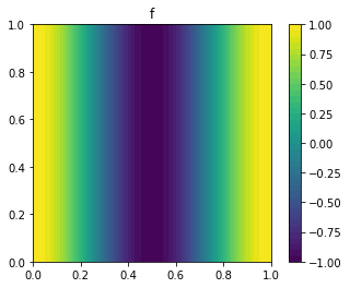
I want to implement fractional Laplacian operator (- \Delta)^{s}. Consider the example problem ( -\Delta)^{s} u(x)= f(x). For f(x)= cos (2 \pi x ), we have the exact solution u_{exact}(x)=cos(2 \pi x)/(2 \pi)^{2 s}.

Below is a code for above example problem that I came up using GitHub - MiroK/hsmg: multigrid for fractional Laplacian. Numerically obtained u(x) and exact solution u_{exact}(x) are matching.

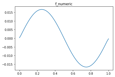
However, numerically obtained f_{numeric}(x) by applying ( -\Delta)^{s} operator on u(x) does not match with the known f(x) (see plots).
(I am using Dirichelt boundary condition as an example for obtaining preconditioner matrix B.)

How to correctly implement fractional Laplacian operator?

from dolfin import *
from hsmg.hseig import HsNorm
from hsmg.hsquad import InvFLaplace
from block.iterative import ConjGrad

s=0.4 # fractional order of differentiation
n=30  # mesh size

mesh = UnitSquareMesh(n, n)      
V = FunctionSpace(mesh, "CG", 1)        

#### forcing function f in RHS
f_expression = Expression('cos(2*pi*x[0])',  degree=2)
f= interpolate(f_expression, V)

#### Exact solution u_exact
u_exact_expression = Expression(' cos(2*pi*x[0]) / pow(2*pi, 2*s) ', s=s, degree=2)
u_exact= interpolate(u_exact_expression, V)

#### numerical solution uh
A = HsNorm(V, s)
bcs= DirichletBC(V, Constant(0), 'on_boundary')
B = InvFLaplace(V, s, bcs, compute_k=0.5)
Ainv = ConjGrad(A, precond=B, tolerance=1E-10)
b = assemble(inner(TestFunction(V), f)*dx)
uh = Function(V, Ainv*b)

#### numerically evaluated f
b2 = assemble(inner(TestFunction(V), uh)*dx)
f_numeric=  Function(V, A*b2)
print( errornorm(f, f_numeric, 'L2') )

[francesco-ballarin]

The most visible difference (apart from the order of magnitude difference) seems to be due to the boundary conditions bcs= DirichletBC(V, Constant(0), 'on_boundary'). Are you sure you really need to apply them?

[pkhandag]

If I remove boundary condition and obtain Ainv matrix as
Ainv = ConjGrad(A, tolerance=1E-10) , I still get the same f_{numeric} as with Dirichelt boundary condition.
If I apply periodic boundary condition on function space V, I do get f_{numeric} that qualitatively matches with f, but the order of magnitude difference between f_{numeric} and f is still the same.

[Stein]

Not sure if I fully understand your code, but is this correct?

@pkhandag

#### numerically evaluated f
b2 = assemble(inner(TestFunction(V), uh)*dx)
f_numeric=  Function(V, A*b2)

Wouldn’t you just need b2 as the vector of dofs from uh? That’s not the same as taking the inner product with a test function.

[pkhandag]

Thanks @Stein. I am not sure how to correctly obatin f_numeric.
When I change Ainv matrix as
Ainv = ConjGrad(A, tolerance=1E-10) , and f_numeric as
f_numeric= Function(V, A*uh.vector()) , the difference in magnitude for f_{numeric} and f has changed to about 10^3 but it still persists (plots attached).

In the source code (line 347 and 356) in the link hsmg/hsmg/hseig.py at master · MiroK/hsmg · GitHub , there is a factor mu=10^4 being used. I am not sure if the error in magnitude of f_numeric and f that I am getting is related to this.

[Stein]

You’re one step closer, but I think the confusion between functions and dof vectors still persists.

A*uh.vector() is definitely the right way to operate on A, but it gives you the right hand side vector, not f. Putting those values as dofs for a function in V still does not give you f.

To reconstruct f, you’d need to solve for the problem:
M*f_reconstruct = A*uh_vector()

With M the L2 inner product matrix, i.e., mass matrix.

I’d imagine you’d still not be able to reconstruct f on the ring of elements at the domain boundary, as the BC there conflicts per the earlier comment

[pkhandag]

How to write M matrix and solve M*f_reconstruct = A*uh_vector() ?
Not sure if M matrix is the same one used in HsNorm function (line 233) in hsmg/hsmg/hseig.py at master · MiroK/hsmg · GitHub

I tried below, but the order of magnitude difference in f and f_numeric still persists.

########### get M and Minv
u1, v1 = TrialFunction(V), TestFunction(V)
m = inner(u1, v1)*dx
# M = assemble (m)

zero = Constant(np.zeros(v1.ufl_element().value_shape()))
L = inner(zero, v1)*dx
M, _ = assemble_system(m, L)

Minv = ConjGrad(M,  tolerance=1E-10)

######### reconstructing f
f_numeric_tmp = Function(V, A*uh.vector())
b2 = assemble(inner(TestFunction(V), f_numeric_tmp)*dx)

f_numeric = Function(V, Minv*b2)

print( errornorm(f, f_numeric, 'L2') )

[Stein]

Like this:
f_numeric = Function(V, Minv*A*uh.vector())

But to be honest, this is not a very useful exercise. This will not tell you whether or not A is a properly implemented fractional laplacian, as the above will always reconstruct f irrespective of what PDE A encodes.

You’d be better off creating a benchmark problem where you know the exact solution, and comparing against that.

[pkhandag]

f_numeric = Function(V, Minv*A*uh.vector()) gives me below error.
I am using the benchmark problem in my 1st post to verify the implementation of fractional Laplacian using A matrix where I am using A = HsNorm(V, s).
The solution uh that I obtain for fractional Laplacian equation in my 1st post matches exactly with truth solution u_exact, so I am assuming at least implementation of inverse of fractional Laplacian using Ainv is correct.

I am considering f used in my 1st post as the truth and comparing reconstructed f_numeric with f to check implementation of fractional Laplacian.

Error message:
File “/home/pratik/anaconda3/envs/fenics19/lib/python3.7/site-packages/block/block_compose.py”, line 46, in mul
if isinstance(op, (GenericMatrix, PETScMatrix, Matrix)) and isinstance(x, (GenericVector, PETScVector, Vector)):

NameError: name ‘PETScMatrix’ is not defined

[urbi95]

Hi, I think the issue is all in the boundary conditions. In your example for u_{exact} I am guessing you assume homogeneous Neumann boundary conditions? Even then, I think the solution might not be unique (that is, adding a constant to u_{exact} would still give you a solution). So that might cause issues later with your operator not being invertible.
But the main point I want to make is that you use hsmg.hseig.HsNorm, but looking at the code on the GitHub page I think they are only considering Dirichlet boundary conditions. That would explain why the result (using Dirichlet bcs) does not match what your expected solution (using Neuman bcs). Hope that answers some questions, even though for a solution you’ll probably have to implement the fractional Laplacian yourself…

[pkhandag]

Thanks @urbi95.
I changed the boundary condition to zero Dirichlet and for simplicity, I chose 1D domain as x \in [0,1]. I also chose f(x)=sin(2\pi x) for which the exact solution would be u_{exact}= sin(2πx)/(2π)^{2s} (I assume it is correct?). Now, both f(x) and u_{exact}(x) satisfy the specified zero Dirichlet boundary condition. Below is the code for this setting. u_exact and solution uh matches. But I am still getting difference in magnitudes of f and reconstructed f_numeric (see plots). The error seems to be in some scaling factor (is it through matrix M?) but I am not sure where.
If I make mesh finer or increase the order of finite element, the error in magnitude of f and f_numeric increases.

import numpy as np
from dolfin import *
from hsmg.hseig import HsNorm
from hsmg.hsquad import InvFLaplace
from block.iterative import ConjGrad

s=0.4 # fractional order of differentiation
n=60  # mesh size

mesh = UnitIntervalMesh(n)
V = FunctionSpace(mesh, "CG", 1)        

#### forcing function f in RHS
f_expression = Expression('sin(2*pi*x[0])',  degree=2)
f= interpolate(f_expression, V)

#### Exact solution u_exact
u_exact_expression = Expression(' sin(2*pi*x[0]) / pow(2*pi, 2*s) ', s=s, degree=2)
u_exact= interpolate(u_exact_expression, V)

#### numerical solution uh
bcs= DirichletBC(V, Constant(0), 'on_boundary')
A = HsNorm(V, s, bcs)
Ainv = ConjGrad(A,  tolerance=1E-10)

b = assemble(inner(TestFunction(V), f)*dx)
uh = Function(V, Ainv*b)

########### get M and Minv
u1, v1 = TrialFunction(V), TestFunction(V)
m = inner(u1, v1)*dx

zero = Constant(np.zeros(v1.ufl_element().value_shape()))
L = inner(zero, v1)*dx
M, _ = assemble_system(m, L)
Minv = ConjGrad(M,  tolerance=1E-10)

######### reconstructing f
f_numeric_tmp = Function(V, A*uh.vector())
b2 = assemble(inner(TestFunction(V), f_numeric_tmp)*dx)

f_numeric = Function(V, Minv*b2)
print( errornorm(f, f_numeric, 'L2') )

[Stein]

I don’t have hsmg or block installed, so I can’t edit your code, but here is a MWE of a regular Poisson equation that is purely fenics. I tried mimicking a bit how you use matrices instead of forms. You can probably extract your necessary ingredients from it:

from dolfin import *
import matplotlib.pyplot as plt

n=30  # mesh size

mesh = UnitSquareMesh(n, n)      
V = FunctionSpace(mesh, "CG", 1)        

#### forcing function f in RHS
f_expression = Expression('cos(2*pi*x[0])',  degree=4)
f = interpolate(f_expression, V)

u_expression = Expression('1/(2*pi*2*pi)*cos(2*pi*x[0])',  degree=4)
u_exact = interpolate(u_expression, V)

#### numerical solution uh
bc_u = DirichletBC(V, u_expression, 'on_boundary')

u, v = TrialFunction(V), TestFunction(V)
a = inner(grad(u), grad(v)) * dx
L = inner(f, v) * dx
uh = Function(V)
solve(a == L, uh, bc_u)
print( "Confirm correctly solved u:", errornorm(u_exact, uh, 'L2') )

A = as_backend_type(assemble(a)).mat()
f_vector = PETScVector(A*uh.vector().vec())

m = inner(u, v)*dx
M = as_backend_type(assemble(m)).mat()
M = assemble(m)

f_numeric = Function(V)
solve(M,f_numeric.vector(),f_vector)

plot(f)
plt.show()
plot(f_numeric)
plt.show()

print( "Confirm correctly reconstructed f:", errornorm(f, f_numeric, 'L2') )

I am honestly a bit surprised by how poorly f is reconstructed, but it converges with the number of elements, so I think it is correct.

Note that I chose Dirichlet BCs compatable with the forcing function (per some of the earlier comments). That is quite important. Try changing that to Constant(0), and you’ll see the reconstructed f differs quite substantially. You can look for ‘lifting operator’ in FEM to try and understand that. Essentially, the impact of the Dirichlet BCs becomes precisely the additional forcing required to ensure the condition.

But my earlier comment stands: This is not a valid way of confirming the validity of your fractional Laplacian implementation. The above will reconstruct f regardless of the weak form that generates A.
But… you already confirmed the validity of the fractional Laplacian implementation by testing that the analytical solution for u is obtained. That is the real confirmation that the implementation is correct. Not some reconstruction of f.