Having difficulty creating 2D streamlines

I wanted to create streamlines out of a vector I created like how it’s done in the streamlines example in the documentation, but in 2D. I heavily utilized the code from the electromagnetics example to create my 2D vector. In fact, you could probably treat this question as also being “how to create streamlines from B in the electromagnetics example?” and that would likely also work for my case. The only differences between that case and mine is that my Poisson’s Equation is simpler and I’m taking the gradient of the solution, rather than the curl. All of my code up to where the issue is occurring is below:

from dolfinx import default_scalar_type
from dolfinx.fem import dirichletbc, Expression, Function, functionspace, locate_dofs_topological, Constant, locate_dofs_topological
from dolfinx.fem.petsc import LinearProblem
from dolfinx.io import XDMFFile
from dolfinx.io.gmshio import model_to_mesh
from dolfinx.mesh import compute_midpoints, locate_entities_boundary, create_rectangle, CellType, exterior_facet_indices
from dolfinx.plot import vtk_mesh

from ufl import TestFunction, TrialFunction, as_vector, dot, dx, grad, inner
from mpi4py import MPI

import numpy as np
import pyvista as pv

# Define mesh
N,M = 5, 5
bounds = [[0.0, 0.0], [1.0, 1.0]]
domain = create_rectangle(MPI.COMM_WORLD, bounds, [N, M],cell_type=CellType.quadrilateral)

# Define functionspace for u and s
V = functionspace(domain, ("Lagrange", 1))
# Define BCs
tdim = domain.topology.dim 
fdim = domain.topology.dim-1 
facets = locate_entities_boundary(domain, tdim - 1, lambda x: np.full(x.shape[1], True))
dofs = locate_dofs_topological(V, tdim - 1, facets)
bc = dirichletbc(default_scalar_type(0), dofs, V)

# Define trial and test functions
u = TrialFunction(V)
s = TestFunction(V)

# Define source
f = Constant(domain, default_scalar_type(-4))

# Define variational form and solve 
a = dot(grad(u),grad(s)) * dx
L = f*s*dx
chi = Function(V)
problem = LinearProblem(a, L, u = chi, bcs= [bc])
chi = problem.solve() # Velocity potential

# Define Gradient of solution
W = functionspace(domain, ("DG",0, (domain.geometry.dim,)),) # Create new function space, make it discontinuous unlike V, and 1 order lower than V
vc = Function(W) # Instantiate function on W functionspace
vc_expr = Expression(as_vector((chi.dx(0),chi.dx(1))),W.element.interpolation_points()) # Create Expression
vc.interpolate(vc_expr) # Interpolate expression onto function

# Reshaping chi and vc values
num_dofs = W.dofmap.index_map.size_local
num_verts = W.mesh.topology.index_map(0).size_local
values = np.zeros((num_dofs, 3), dtype=np.float64)
values[:, :domain.geometry.dim] = vc.x.array.real.reshape(num_dofs, W.dofmap.index_map_bs)
values2 = np.zeros((num_verts, 3), dtype=np.float64)
values2[:, :domain.geometry.dim] = chi.x.array.real.reshape(num_verts, V.dofmap.index_map_bs)

# Assign v and vc onto grid
grid = pv.UnstructuredGrid(*vtk_mesh(domain, tdim))
grid.point_data["chi"] = chi.x.array.real
grid.set_active_scalars("chi")
grid["vc"] = values
grid.set_active_vectors("vc")
glyphs = grid.glyph(orient = "vc", scale = "vc", factor = .1)  # vc vectors

# Assign streamlines to grid
streamlines = grid.streamlines(vectors="vc", return_source=False, source_radius=0.5)

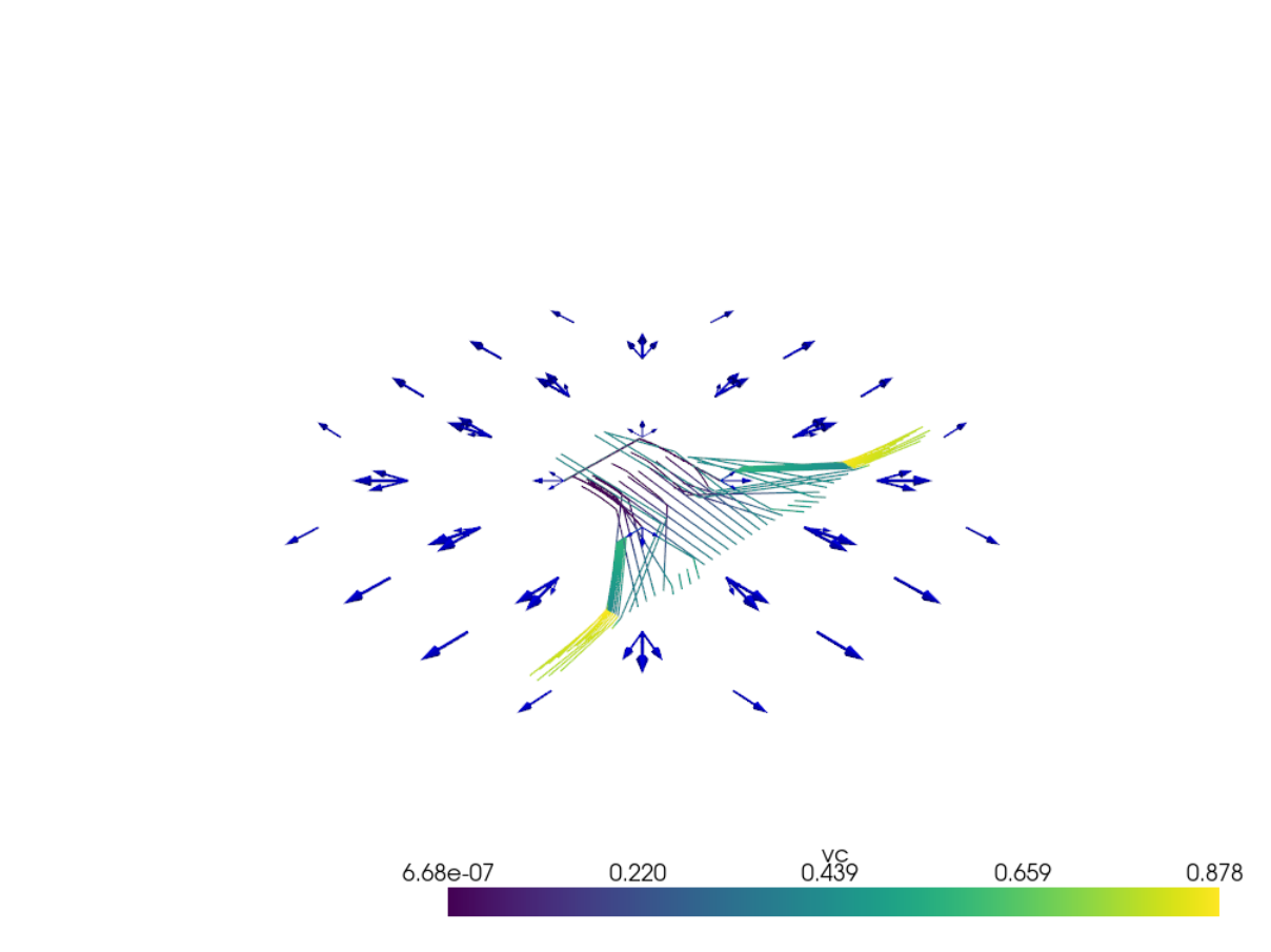
The last line where I attempt to create streamlines out of the vectors returns an empty mesh each time. Here’s a plot of the scalars and glyphs I was successfully able to create below:

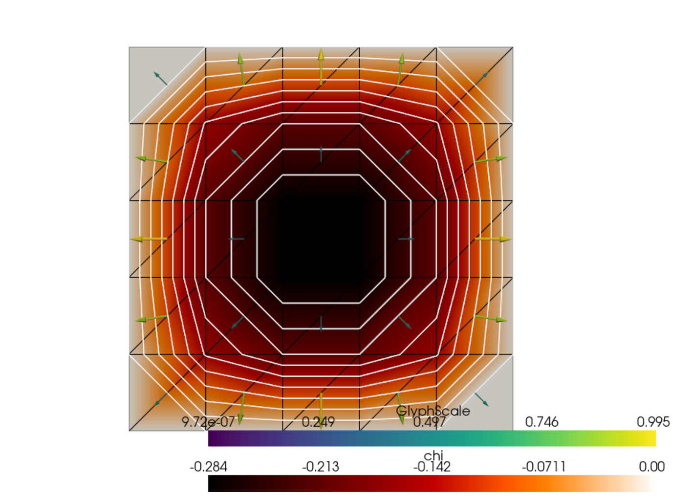
If I can create the streamlines, I’m expecting them to be parallel with and go through the arrows pointing away from the center. Should be 16 streamlines in total pointing out from the center.

You are using the wrong function space for vc.
As you have created your pyvista grid from the mesh, and associate data with the vertices of the mesh, even if it is cell data.
Additionally, there are issues with using streamlines in 2D, you can’t use a ball-source, and have to provide the linea and lineb arguments.
Here you have an illustration of partial streamlines using this kind of structure and a DG-1 space:

from dolfinx import default_scalar_type
from dolfinx.fem import (
    dirichletbc,
    Expression,
    Function,
    functionspace,
    locate_dofs_topological,
    Constant,
    locate_dofs_topological,
)
from dolfinx.fem.petsc import LinearProblem
from dolfinx.io import XDMFFile
from dolfinx.io.gmshio import model_to_mesh
from dolfinx.mesh import (
    compute_midpoints,
    locate_entities_boundary,
    create_rectangle,
    CellType,
    exterior_facet_indices,
)
from dolfinx.plot import vtk_mesh

from ufl import TestFunction, TrialFunction, as_vector, dot, dx, grad, inner
from mpi4py import MPI

import numpy as np
import pyvista as pv

# Define mesh
N, M = 5, 5
bounds = [[0.0, 0.0], [1.0, 1.0]]
domain = create_rectangle(
    MPI.COMM_WORLD, bounds, [N, M], cell_type=CellType.quadrilateral
)

# Define functionspace for u and s
V = functionspace(domain, ("Lagrange", 1))
# Define BCs
tdim = domain.topology.dim
fdim = domain.topology.dim - 1
facets = locate_entities_boundary(domain, tdim - 1, lambda x: np.full(x.shape[1], True))
dofs = locate_dofs_topological(V, tdim - 1, facets)
bc = dirichletbc(default_scalar_type(0), dofs, V)

# Define trial and test functions
u = TrialFunction(V)
s = TestFunction(V)

# Define source
f = Constant(domain, default_scalar_type(-4))

# Define variational form and solve
a = dot(grad(u), grad(s)) * dx
L = f * s * dx
chi = Function(V)
problem = LinearProblem(a, L, u=chi, bcs=[bc])
chi = problem.solve()  # Velocity potential

# Define Gradient of solution
W = functionspace(
    domain,
    ("DG", 1, (domain.geometry.dim,)),
)  # Create new function space, make it discontinuous unlike V, and 1 order lower than V
vc = Function(W)  # Instantiate function on W functionspace
vc_expr = Expression(
    as_vector((chi.dx(0), chi.dx(1))), W.element.interpolation_points()
)  # Create Expression
vc.interpolate(vc_expr)  # Interpolate expression onto function

# Reshaping chi and vc values
num_dofs = W.dofmap.index_map.size_local
num_verts = W.mesh.topology.index_map(0).size_local
values = np.zeros((num_dofs, 3), dtype=np.float64)
values[:, : domain.geometry.dim] = vc.x.array.real.reshape(
    num_dofs, W.dofmap.index_map_bs
)
values2 = np.zeros((num_verts, 3), dtype=np.float64)
values2[:, : domain.geometry.dim] = chi.x.array.real.reshape(
    num_verts, V.dofmap.index_map_bs
)

# Assign v and vc onto grid
W0, _ = W.sub(0).collapse()
grid = pv.UnstructuredGrid(*vtk_mesh(W))
chi_out = Function(W0)
chi_out.interpolate(chi)  # Interpolate chi onto W
grid.point_data["chi"] = chi_out.x.array
grid.set_active_scalars("chi")
grid.point_data["vc"] = values
grid.set_active_vectors("vc")
glyphs = grid.glyph(orient="vc", scale="vc", factor=0.1)  # vc vectors

# Assign streamlines to grid

plotter = pv.Plotter()
plotter.add_mesh(glyphs, color="blue")
streamlines = grid.streamlines(
    vectors="vc",
    pointa=(0.0, 0.75, 0),
    pointb=(1, 0.75, 0),
    return_source=False,
    n_points=50,
)

plotter.add_mesh(streamlines)
# pv.start_xvfb(0.5)
plotter.show()
1 Like

There’s only one issue now, and this is a new one, it looks like there are some vectors we don’t want or need. Should just be 1 vector like in the original image (except with each vector being centered at the vertices). You can see that in the image below:

It looks to me like the middle vectors among the 3 vectors at each vertex are the correct ones.

I’m parsing through it, and since the grid created using the functionspace accepts arrays of shape (100,3) or (100,), and the original solution chi has array data of shape (36,), I kinda have to create an interpolated definition chi_out even though this presents an issue of the extra vectors onto each point coming from the larger size of its respective array. Maybe I should create 2 separate grids and plot arrays and streamlines separately using different grids? What are your thoughts?

Streamlines and discontinuous fields remains a bit challenging, as long as VTKDGCellDiscontinuous Galerkin Support in Paraview - ParaView Support - ParaView only has partial support in pyvista and paraview.

A partial workaround is to change

to

W = functionspace(
    domain,
    ("CG", 1, (domain.geometry.dim,)),
)

even if this would introduce a “variational” crime/inconsistency.

Resulting plot:

1 Like

Yeah that’s about exactly what I was looking for. Thank you!