How to apply boundary conditions when using petsc4py.PETSc.SNES directly?

wolfj · May 28, 2021, 8:38am

Hello everyone,

I am currently trying to solve a nonlinear problem by using petsc4py.PETSc.SNES directly. The problem is a 2D unit square with a neo-Hooke material and a traction applied to the right boundary. I followed the code given by niewiarowski and nate:
https://fenicsproject.discourse.group/t/using-petsc4py-petsc-snes-directly/2368

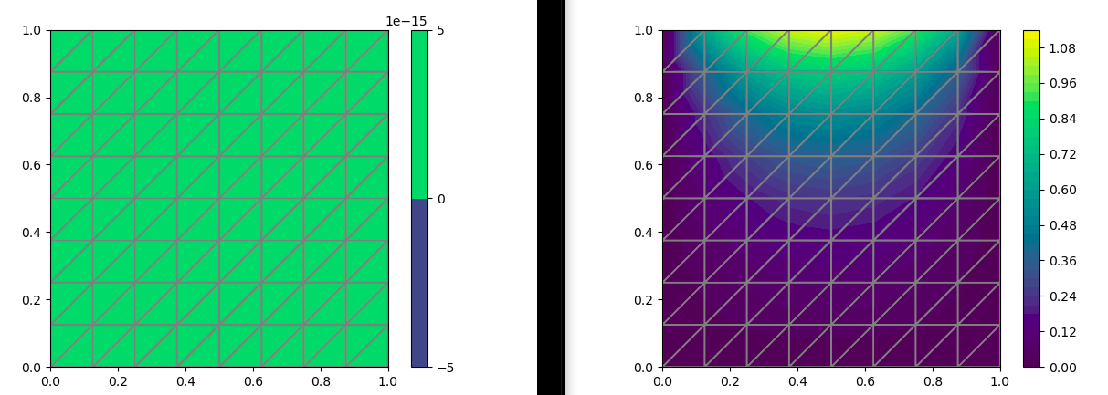
I encounter a problem when it comes to the boundary conditions: Everything seems to work fine when I set a non-homogeneous Dirichlet-BC (e.g. a displacement of (0,0.1) ) to the left boundary. However, when I set a zero-displacement Dirichlet-BC to the left boundary, the solution shows a zero-displacement in the whole domain, ignoring the traction set to the right side.

Here is a picture of the solution field, on the left with the non-zero Dirichlet-BC and on the right with the zero Dirichlet-BC:

Here is the MWE:

import dolfin as dlf
import numpy as np
import petsc4py, sys
petsc4py.init(sys.argv)
from petsc4py import PETSc
import matplotlib.pyplot as plt

# Elasticity parameters
E, nu = 10.0, 0.3
mu, lmbda = dlf.Constant(E/(2*(1 + nu))), dlf.Constant(E*nu/((1 + nu)*(1 - 2*nu)))
# boundary displacement
u0 = dlf.Constant((0, 0))
# u0 = dlf.Constant((0, 0.1)) # with this u0, everything seems to work
# boundary traction
t0 = dlf.Constant((0.0, 0.1))
# volume force
f = dlf.Constant((0.0, 0.0))

# define boundaries
def left(x, on_boundary):
    return on_boundary and dlf.near(x[0], 0.0)

def right(x, on_boundary):
    return on_boundary and dlf.near(x[0], 1)

mesh=dlf.UnitSquareMesh(16,16)

# define function space
V = dlf.VectorFunctionSpace(mesh, 'P', 1)

# define Dirichlet (displacement) boundary conditions
bcleft = dlf.DirichletBC(V, u0, left)
bcs = [bcleft]

#define Neumann (traction) boundary conditions
traction_markers = dlf.MeshFunction('size_t', mesh, mesh.topology().dim()-1)
traction_markers.set_all(0)
traction_domain = dlf.AutoSubDomain(right)
traction_domain.mark(traction_markers, 1)
ds_t = dlf.ds(subdomain_data=traction_markers)(1)

# define variational problem
u = dlf.Function(V)
v = dlf.TestFunction(V)
du = dlf.TrialFunction(V)

# Kinematics
d = u.geometric_dimension()
I = dlf.Identity(d)             # Identity tensor
F = I + dlf.grad(u)             # Deformation gradient
C = F.T*F
# Invariants of deformation tensors
Ic = dlf.tr(C)
J  = dlf.det(F)

# Stored strain energy density (compressible neo-Hookean model)
psi = (mu/2)*(Ic - 3) - mu*dlf.ln(J) + (lmbda/2)*(dlf.ln(J))**2

# Total potential energy
Pi = psi*dlf.dx - dlf.dot(f, u)*dlf.dx - dlf.dot(t0, u)*ds_t

# Compute first variation of Pi (directional derivative about u in the direction of v)
Var = dlf.derivative(Pi, u, v)
#Jac = dlf.derivative(Var, u, du)

class SNESProblem():
    def __init__(self, F, u, bcs):
        V = u.function_space()
        du = dlf.TrialFunction(V)
        self.L = F
        self.a = dlf.derivative(F, u, du)
        self.bcs = bcs
        self.u = u

    def F(self, snes, x, F):
        x = dlf.PETScVector(x)
        F  = dlf.PETScVector(F)
        dlf.assemble(self.L, tensor=F)
        for bc in self.bcs:
            bc.apply(F, x)

    def J(self, snes, x, J, P):
        J = dlf.PETScMatrix(J)
        dlf.assemble(self.a, tensor=J)
        for bc in self.bcs:
            bc.apply(J)

problem = SNESProblem(Var, u, bcs)

b = dlf.PETScVector()
J_mat = dlf.PETScMatrix()

snes = PETSc.SNES().create(dlf.MPI.comm_world)
snes.setFunction(problem.F, b.vec())
snes.setJacobian(problem.J, J_mat.mat())
snes.setFromOptions()
snes.solve(None, problem.u.vector().vec())

uconv = u((1,1))

print('')
print(' Reporting results ...')
print(' v(1/1) = ', uconv[1])

# Plot and hold solution
pu=dlf.plot(u, mode='displacement')
plt.colorbar(pu)
plt.show()

I am using the dolfin version 2019.2.0.dev.

Any help would be greatly appreciated!
Jana

wolfj · June 7, 2021, 1:51pm

@niewiarowski, @nate maybe you can help?

niewiarowski · June 14, 2021, 7:17pm

Hi, did you manage to figure this out?

wolfj · June 15, 2021, 6:45am

Hi! No, unfortunately not… Do you have any ideas?

dokken · June 15, 2021, 7:28am

An illustration of how to use snes with bcs in dolfinx is shown: dolfinx/test_nonlinear_assembler.py at main · FEniCS/dolfinx · GitHub

niewiarowski · June 15, 2021, 8:25pm

I tried a few things but nothing immediately comes to mind. It’s interesting that u0 = dlf.Constant((0, 1e-5)) doesn’t work but u0 = dlf.Constant((0, 1e-4)) does. Can you replicate this issue with another problem?

wolfj · June 21, 2021, 12:10pm

@dokken thanks for the reference. I am considering to switch to dolfinx for this problem.
@niewiarowski it took me some time, but I managed to replicate the issue with a Poisson problem. I am using u_D as a constant Dirichlet BC on the left, right and bottom boundary and applying a Neumann BC on the top of the domain. The results look like this (left: u_D=Constant(0), right: u_D=Constant(1e-3). In this example, u_D=Constant(1e-4) doesn’t work anymore.

When playing around with this example, I compared it to the results of an implementation of the same problem, but with the standard usage of SNES via solver.parameters['nonlinear_solver']='snes' and NonlinearVariationalProblem. The results are not the same - e.g. if I choose u_D=Constant(0.1), I get a result of u(0.5,0.5) = 0.4201732544314507 for the direct implementation of SNES and u(0.5,0.5) = 0.26009739812490046 for the standard one.
I attach both codes here and would be happy to hear any ideas.

Code where I try to use SNES directly

from fenics import *
import matplotlib.pyplot as plt
import petsc4py, sys
petsc4py.init(sys.argv)
from petsc4py import PETSc
import matplotlib.pyplot as plt

# Create mesh and define function space
mesh = UnitSquareMesh(8, 8)
V = FunctionSpace(mesh, 'P', 2)

# Define boundary condition
#u_D = Expression('1 + x[0]*x[0] + 2*x[1]*x[1]', degree=2)
u_D=Constant(0.1)

def left(x, on_boundary):
    return on_boundary and near(x[0], 0.0)
def right(x, on_boundary):
    return on_boundary and near(x[0], 1.0)
def bottom(x, on_boundary):
    return on_boundary and near(x[1], 0.0)
def top(x, on_boundary):
    return on_boundary and near(x[1], 1.0)

bc_left = DirichletBC(V, u_D, left)
bc_right = DirichletBC(V, u_D, right)
bc_bottom = DirichletBC(V, u_D, bottom)
bc_top = DirichletBC(V, u_D, top)
bcs=[bc_left,bc_right,bc_bottom]

# Define variational problem
u = Function(V)
v = TestFunction(V)
#f = Constant(-6.0)
f=Constant(0)
a = dot(grad(u), grad(v))*dx
g_s=Constant(2)
L = f*v*dx+g_s*v*ds
F = a-L


class SNESProblem():
    def __init__(self, F, u, bcs):
        V = u.function_space()
        du = TrialFunction(V)
        self.L = F
        self.a = derivative(F, u, du)
        self.bcs = bcs
        self.u = u

    def F(self, snes, x, F):
        x = PETScVector(x)
        F  = PETScVector(F)
        assemble(self.L, tensor=F)
        for bc in self.bcs:
            bc.apply(F, x)

    def J(self, snes, x, J, P):
        J = PETScMatrix(J)
        assemble(self.a, tensor=J)
        for bc in self.bcs:
            bc.apply(J)

problem = SNESProblem(F, u, bcs)

b = PETScVector()
J_mat = PETScMatrix()

snes = PETSc.SNES().create(MPI.comm_world)
snes.setFunction(problem.F, b.vec())
snes.setJacobian(problem.J, J_mat.mat())
snes.setFromOptions()
snes.solve(None, problem.u.vector().vec())

uconv = u((0.5,0.5))

print('')
print(' Reporting results ...')
print(' u(0.5,0.5) = ', uconv)

# Plot solution and mesh
pu=plot(u)
plot(mesh)
plt.colorbar(pu)
plt.show()

Code with SNES as a parameter:

from fenics import *
import matplotlib.pyplot as plt

# Create mesh and define function space
mesh = UnitSquareMesh(8, 8)
V = FunctionSpace(mesh, 'P', 2)

# Define boundary condition
#u_D = Expression('1 + x[0]*x[0] + 2*x[1]*x[1]', degree=2)
u_D=Constant(0.1)

def boundary(x, on_boundary):
    return on_boundary

def left(x, on_boundary):
    return on_boundary and near(x[0], 0.0)
def right(x, on_boundary):
    return on_boundary and near(x[0], 1.0)
def bottom(x, on_boundary):
    return on_boundary and near(x[1], 0.0)
def top(x, on_boundary):
    return on_boundary and near(x[1], 1.0)

bc_left = DirichletBC(V, u_D, left)
bc_right = DirichletBC(V, u_D, right)
bc_bottom = DirichletBC(V, u_D, bottom)
bc_top = DirichletBC(V, u_D, top)
bcs=[bc_left,bc_right,bc_bottom]

# Define variational problem
u = Function(V)
v = TestFunction(V)
#f = Constant(-6.0)
f=Constant(0)
a = dot(grad(u), grad(v))*dx
g_s=Constant(2)
L = f*v*dx+g_s*v*ds
F = a-L

# Compute solution
Jac = derivative(F,u)
problem = NonlinearVariationalProblem(F,u,bcs,Jac)
solver=NonlinearVariationalSolver(problem)
solver.parameters['nonlinear_solver']='snes'
solver.solve()

uconv = u((0.5,0.5))

print('')
print(' Reporting results ...')
print(' u(0.5,0.5) = ', uconv)

# Plot solution and mesh
pu=plot(u)
plot(mesh)
plt.colorbar(pu)
plt.show()

Topic		Replies	Views
Using petsc4py.PETSc.SNES directly Linear Algebra	23	4580	June 13, 2024
Initial and Boundary Conditions General	3	229	May 12, 2023
How to implement problem with only Neumann BCs, no Dirichlet	1	279	September 7, 2023
Some issues with snes_solvers General	2	47	April 29, 2025
Custom Newton Solver problem with Dirichlet conditions	16	4351	January 31, 2024

How to apply boundary conditions when using petsc4py.PETSc.SNES directly?

Related topics