Hello everyone,
I am trying to solve a heat conduction problem on 2 submeshes using mixed dimensional branch. However, I would like to use the lower level functions instead of using the high level solve function
solve (a == L, sol , bc)
I have managed to solve the problem by create a new unknown vector and store the solution in that vector (The solution seems to be correct compared to the solution from the high level solve function visulised in ParaView).
Solution from high level solve function
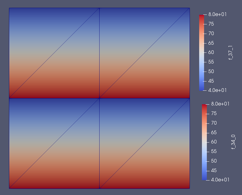
Solution from low level solve function
However, I also need to convert this solution vector back to Function object inorder to visualize the result in ParaView.
Could anyone please suggest how to perform this conversion?
Here is the MWE
from __future__ import print_function
import numpy as np
import matplotlib.pyplot as plt
from dolfin import *
from ufl.algorithms import expand_derivatives
import petsc4py.PETSc as petsc

class Top(SubDomain):
    def inside(self, x, on_boundary):
        return near(x[1], 1.0)

class Left1(SubDomain):
   def inside(self, x, on_boundary):
        return near(x[0], 0.0) and between(x[1], (0.5, 1))

class Right1(SubDomain):
    def inside(self, x, on_boundary):
        return near(x[0], 1.0) and between(x[1], (0.5, 1))

class Interface(SubDomain):
    def inside(self, x, on_boundary):
        return near(x[1], 0.5)

class Left2(SubDomain):
    def inside(self, x, on_boundary):
        return near(x[0], 0.0) and between(x[1], (0.0, 0.5))

class Right2(SubDomain):
    def inside(self, x, on_boundary):
        return near(x[0], 1.0) and between(x[1], (0.0, 0.5))

class Bottom(SubDomain):
    def inside(self, x, on_boundary):
        return near(x[1], 0.0)

# Create meshes
mesh = UnitSquareMesh(2, 2)

# Domain markers
domain = MeshFunction("size_t", mesh, mesh.geometry().dim(), 0)

for c in cells(mesh):
  domain[c] = c.midpoint().y() > 0.5

# Interface markers
facets = MeshFunction("size_t", mesh, mesh.geometry().dim()-1, 0)
Interface().mark(facets,1)

# Define submeshes
mesh_F = MeshView.create(domain, 1)
mesh_S = MeshView.create(domain, 0)

# Function spaces
TE = FiniteElement("CG", mesh.ufl_cell(), 1)   # Temperature
T_F  = FunctionSpace(mesh_F,TE)    # Temperature on the upper domain
T_S  = FunctionSpace(mesh_S,TE)    # Temperature on the lower domain
W = MixedFunctionSpace(T_F, T_S)

# Markers for Dirichlet and Neuman bcs
ff_F = MeshFunction("size_t", mesh_F, mesh_F.geometry().dim()-1, 0)
Top().mark(ff_F, 1)
Left1().mark(ff_F, 2)
Right1().mark(ff_F, 3)
Interface().mark(ff_F, 4)

ff_S = MeshFunction("size_t", mesh_S, mesh_S.geometry().dim()-1, 0)
Interface().mark(ff_S, 5)
Left2().mark(ff_S, 6)
Right2().mark(ff_S, 7)
Bottom().mark(ff_S, 8)

# Boundary conditions
bc_U1 = DirichletBC(W.sub_space(0), Constant(40), ff_F, 1)
bc_U2 = DirichletBC(W.sub_space(0), Constant(80), ff_F, 4)
bc_L1 = DirichletBC(W.sub_space(1), Constant(40), ff_S, 5)
bc_L2 = DirichletBC(W.sub_space(1), Constant(80), ff_S, 8)
bcs = [bc_U1, bc_U2, bc_L1, bc_L2]

# Material parameters
k_f = Constant(227) #Constant(0.5984)
k_s = Constant(0.5984) #Constant(227)

# Measures
dx_F  = Measure("dx", domain=W.sub_space(0).mesh())
ds_F  = Measure("ds", domain=W.sub_space(0).mesh(), subdomain_data=ff_F)
dx_S  = Measure("dx", domain=W.sub_space(1).mesh())
ds_S  = Measure("ds", domain=W.sub_space(1).mesh(), subdomain_data=ff_S)

nf = FacetNormal(mesh_F) # unit normal vector on the surfaces of the fluid mesh
ns = FacetNormal(mesh_S) # unit normal vector on the surfaces of the solid mesh

(tf, ts) = TrialFunctions(W)
(zf, zs) = TestFunctions(W)

# Define the weak form
f = Constant(0.0)

# Variational problem in fluid
a_fluid = k_f*inner(grad(tf), grad(zf))*dx_F
L_fluid = f*zf*dx_F

# Variational problem in solid
a_solid = k_s*inner(grad(ts), grad(zs))*dx_S
L_solid = f*zs*dx_S

# Combined variational problem
a =  a_fluid + a_solid
L =  L_fluid + L_solid

# Define function object
t_mixed = Function(W)
tf = t_mixed.sub(0)
ts = t_mixed.sub(1)

# Assembly and Solve
system = assemble_mixed_system(a == L, t_mixed, bcs)
matrix_blocks = system[0]
rhs_blocks = system[1]

A = PETScNestMatrix(matrix_blocks)
b = Vector()
A.init_vectors(b, rhs_blocks)
A.convert_to_aij()

x = Vector()
solve(A,x,b)
Thank you very much
Phuris


