How to create subdomains(boundaries) of polygonal meshes, and how to assign arrays of values to a boundary?

[fea]

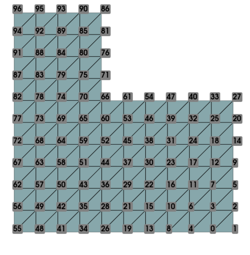
I have 2 questions which arise from wanting to apply Dirichlet boundary conditions to a L-shaped polygon like the one below

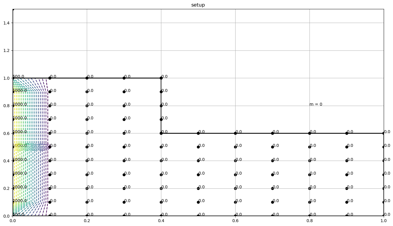
where it can be seen that the boundary values are 0 everywhere except for the left side of the L-shaped grid, where the corner values are 500 and the remaining values are 1000 (ignore the values on the points inside).

1. Creating individual boundaries polygonal mesh?

I’ll start off creating the L-shaped mesh (which is the code of another user who had helped me previously) below:

bounds = [[0.0, 0.0], [1.0, 1.0]]  # Original bounds of rectangle
xcutoff, ycutoff = 0.4, 0.6  # Cutoff to make L-shape

mesh = df.mesh.create_rectangle(MPI.COMM_WORLD, bounds, [10, 10])

tdim = mesh.topology.dim
im_tdim = mesh.topology.index_map(tdim)
cells = np.arange(im_tdim.size_local + im_tdim.num_ghosts, dtype=np.int32)
midpoints = df.mesh.compute_midpoints(mesh, tdim, cells)
cells_to_remove = (midpoints[:, 0] >= xcutoff) & (midpoints[:, 1] >= ycutoff)
cells_to_keep = np.where(~cells_to_remove)[0]
lmesh, _, _, _ = df.mesh.create_submesh(mesh, mesh.topology.dim, cells_to_keep)

And following the tutorial to create boundaries and attempting to apply this for an L-shaped block:

# Define the boundaries
boundaries = [(1, lambda x: np.isclose(x[0], 0)), #(marker = 1, locator = (x=0,y=y))
              (2, lambda x: np.isclose(X[0],0.4) & np.greater_equal(X[1],0.6)), #(marker = 2, locator = (x=0.4,y>=0.6))
              (3, lambda x: np.isclose(x[0], 1)), #(marker = 3, locator = (x=1,y=y))
              (4, lambda x: np.isclose(x[1], 0)), #(marker = 4, locator = (x=x,y=0))
              (5, lambda x: np.isclose(X[1],0.6) & np.greater_equal(X[0],0.4)), #(marker = 5, locator = (x>=0.4,y=0.6))
              (6, lambda x: np.isclose(x[1], 1))] #(marker = 6, locator = (x=x,y=1))

My definitions for boundaries 2 and 5 raise issues at the step for identifying the facets which make up the boundaries in the next step

domain = lmesh
facet_indices, facet_markers = [], []
fdim = mesh.topology.dim - 1 # Facet dimensionality 
for (marker, locator) in boundaries:
    facets = df.mesh.locate_entities(domain, fdim, locator)
    facet_indices.append(facets)
    facet_markers.append(np.full_like(facets, marker))

gives the output error when reading in boundary 2:

---------------------------------------------------------------------------
RuntimeError                              Traceback (most recent call last)
Cell In[11], line 4
      2 fdim = mesh.topology.dim - 1 # Facet dimensionality 
      3 for (marker, locator) in boundaries:
----> 4     facets = df.mesh.locate_entities(mesh, fdim, locator)
      5     facet_indices.append(facets)
      6     facet_markers.append(np.full_like(facets, marker))

File ~/anaconda3/envs/fea/lib/python3.13/site-packages/dolfinx/mesh.py:470, in locate_entities(msh, dim, marker)
    456 def locate_entities(msh: Mesh, dim: int, marker: typing.Callable) -> np.ndarray:
    457     """Compute mesh entities satisfying a geometric marking function.
    458 
    459     Args:
   (...)    468         Indices (local to the process) of marked mesh entities.
    469     """
--> 470     return _cpp.mesh.locate_entities(msh._cpp_object, dim, marker)

RuntimeError: Length of array of markers is wrong.

Can my definitions for the boundaries be fixed, or will this require a different approach?

2. Applying an array of values to a boundary?

I want to assign the array of values

vals = np.array([500,1000,1000,1000,1000,1000,1000,1000,1000,1000,500],dtype = 'int32')

to the left boundary to make it the same as in the figure. Previously I have seen how to apply an expression or a constant default_scalar_type(), but not an array of values to explicitly apply to each boundary point. Is there a way to do this?

[fea]

I think I just needed to separate it or perhaps defining the locator via lambda functions wasn’t allowing for multiple conditions, because moving to a user-defined function the following way below worked

def right_handle(x):
    truth_arr = np.greater_equal(x[1],0.6) & np.isclose(x[0],0.4)
    return truth_arr
right_hand_dofs = df.fem.locate_dofs_geometrical(V,right_handle)
print("right handle vertices: ", right_hand_dofs)

prints out

right handle vertices:  [66 71 76 81 86]

which lines up with one of the regions I was trying to isolate as can be seen in the image below showing the map of vertices/degrees of freedom

With that out of the way, I found a more efficient way to tackle this problem by isolating the boundaries that I wanted and utilizing dolfinx.mesh.exterior_facet_indices(). All of my code is provided below along with the plotted solution to Laplace’s Equation on this L-shaped block:

# Define function space
V = df.fem.functionspace(mesh = lmesh, element = ("Lagrange",1))

tdim = lmesh.topology.dim # Dimension of entities one is mapping from
fdim = lmesh.topology.dim-1 # Dimension of entities one is mapping to
# Always remember to establish connectivity between points    
lmesh.topology.create_connectivity(fdim, tdim)

# Start by getting boundary facets (vertices)
boundary_facets = df.mesh.exterior_facet_indices(lmesh.topology)
boundary_dofs = df.fem.locate_dofs_topological(V, fdim, boundary_facets)
print("boundary vertices: ",boundary_dofs)

# Then isolate the boundary vertices with unique values
def left_boundary(x):
    truth_arr = (np.greater(x[1],1E-8) & np.less(x[1],1)) & np.isclose(x[0],0)
    return truth_arr
left_dofs = df.fem.locate_dofs_geometrical(V, left_boundary)
print("left boundary (excluding corners): ", left_dofs)
bc_left = df.fem.dirichletbc(df.default_scalar_type(1000),left_dofs,V) 

def lower_left_corner(x):
    return np.isclose(x[0],0) & np.isclose(x[1],0)
ll_dofs = df.fem.locate_dofs_geometrical(V,lower_left_corner)
bc_ll = df.fem.dirichletbc(df.default_scalar_type(500),ll_dofs,V)
print("lower left corner: ", ll_dofs)

def upper_left_corner(x):
    return np.isclose(x[0],0) & np.isclose(x[1],1)
ul_dofs = df.fem.locate_dofs_geometrical(V,upper_left_corner)
bc_ul = df.fem.dirichletbc(df.default_scalar_type(500),ul_dofs,V)
print("upper left corner: ", ul_dofs)

l_boundary_dofs = ll_dofs.tolist() + left_dofs.tolist() + ul_dofs.tolist()
boundary_dofs = boundary_dofs.tolist()
print("boundary vertices used so far: ", l_boundary_dofs)

# Now create a boundary out of remaining vertices
for dof in boundary_dofs:
    if dof in l_boundary_dofs:
        boundary_dofs.remove(dof)
boundary_dofs = np.asarray(boundary_dofs, dtype = 'int32')
print("remaining boundary vertices: ", boundary_dofs)
bc_remaining = df.fem.dirichletbc(df.default_scalar_type(0),boundary_dofs,V)

# Define Trial and Test functions
u = ufl.TrialFunction(V)
s = ufl.TestFunction(V)

# Define source term
f = df.fem.Constant(lmesh, df.default_scalar_type(0))

# Define terms in abstract variational form
a = ufl.dot(ufl.grad(u),ufl.grad(s)) * ufl.dx
L = f*s*ufl.dx

# use PETSc as our linear algebra backend
from dolfinx.fem.petsc import LinearProblem
problem = LinearProblem(a=a,L=L,bcs = [bc_ll,bc_left,bc_ul,bc_remaining], petsc_options={"ksp_type": "preonly", "pc_type": "lu"}) 
uh = problem.solve()

# Plot solution
grid = pv.UnstructuredGrid(*df.plot.vtk_mesh(V))
grid.point_data["u"] = uh.x.array.real
grid.set_active_scalars("u")
contours = grid.contour(isosurfaces = 21)
plotter = pv.Plotter()
plotter.add_mesh(grid, show_edges=True, show_scalar_bar=True, cmap = 'gist_heat')
plotter.show_grid()
plotter.add_mesh(contours, color ='white')
plotter.view_xy()
plotter.show()