Hi Dolfinx community!
I’m working on a stabilized Navier-Stokes solver using DOLFINx 0.9.0 using equal order interpolation with SUPG and PSPG stabilization. The weak formulation follows the formulation in Donea & Huerta, Finite Element Methods for Flow Problems (2003), Section 6.6.1.
\begin{aligned} F(u, p; v, q) &= \rho \int_{\Omega} \mathbf{v} \cdot \left[(\mathbf{u} \cdot \nabla)\mathbf{u}\right] \, d\Omega + \mu \int_{\Omega} \nabla \mathbf{v} : \nabla \mathbf{u} \, d\Omega \\ &\quad - \int_{\Omega} p \, \nabla \cdot \mathbf{v} \, d\Omega + \int_{\Omega} q \, \nabla \cdot \mathbf{u} \, d\Omega - \rho \int_{\Omega} \mathbf{v} \cdot \mathbf{b} \, d\Omega \\[1em] &\quad + \int_{\Omega} \tau_{\text{SUPG}} \, (\nabla \mathbf{v} \, \mathbf{u}) \cdot \mathbf{R}_m \, d\Omega + \int_{\Omega} \tau_{\text{PSPG}} \, \nabla q \cdot \mathbf{R}_m \, d\Omega \end{aligned}
\mathbf{R}_m = \rho \frac{\partial \mathbf{u}}{\partial t} + \rho (\mathbf{u} \cdot \nabla)\mathbf{u} - \mu \nabla^2 \mathbf{u} + \nabla p - \rho \mathbf{b}
\tau = \left[ (2 \theta / \Delta t)^2 + (2 |\mathbf{u}| / h)^2 + (4 \nu / h^2)^2 \right]^{-1/2}
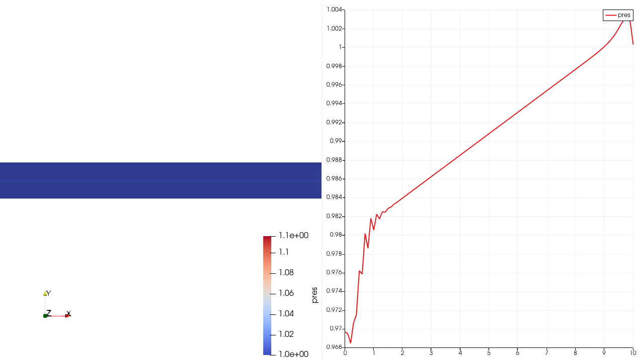
The solver behaves as expected for the velocity field, the soltuion converges quickly to the parabolic profile expected for Poiseuille flow in a 2D channel. However, the pressure field exhibits stong oscillations, especially near the beginning of the simulation (see images below). The solution eventually converges toward the physically correct steady-state, but this is not suitable for unsteady problems where the outlet pressure is prescribed as a transient boundary condition (e.g., modeling physiological outflow or time-dependent traction).
t = 50 steps
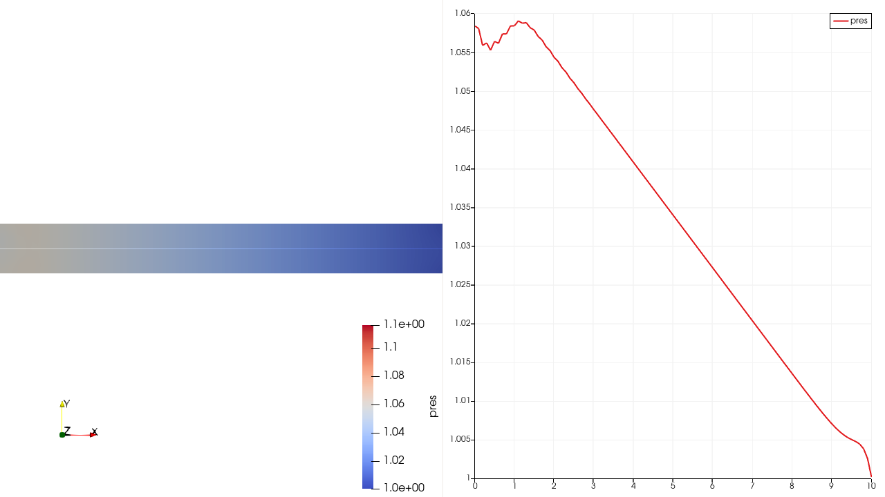
t=150 steps
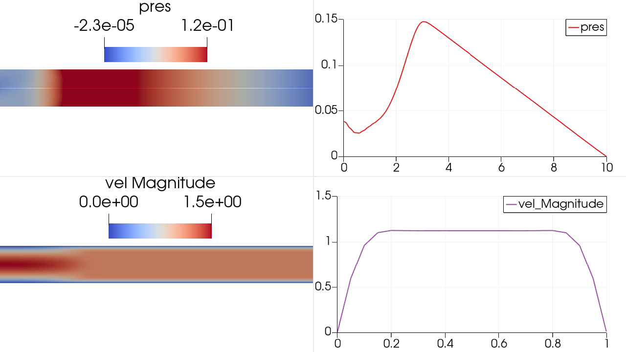
t = 300 steps

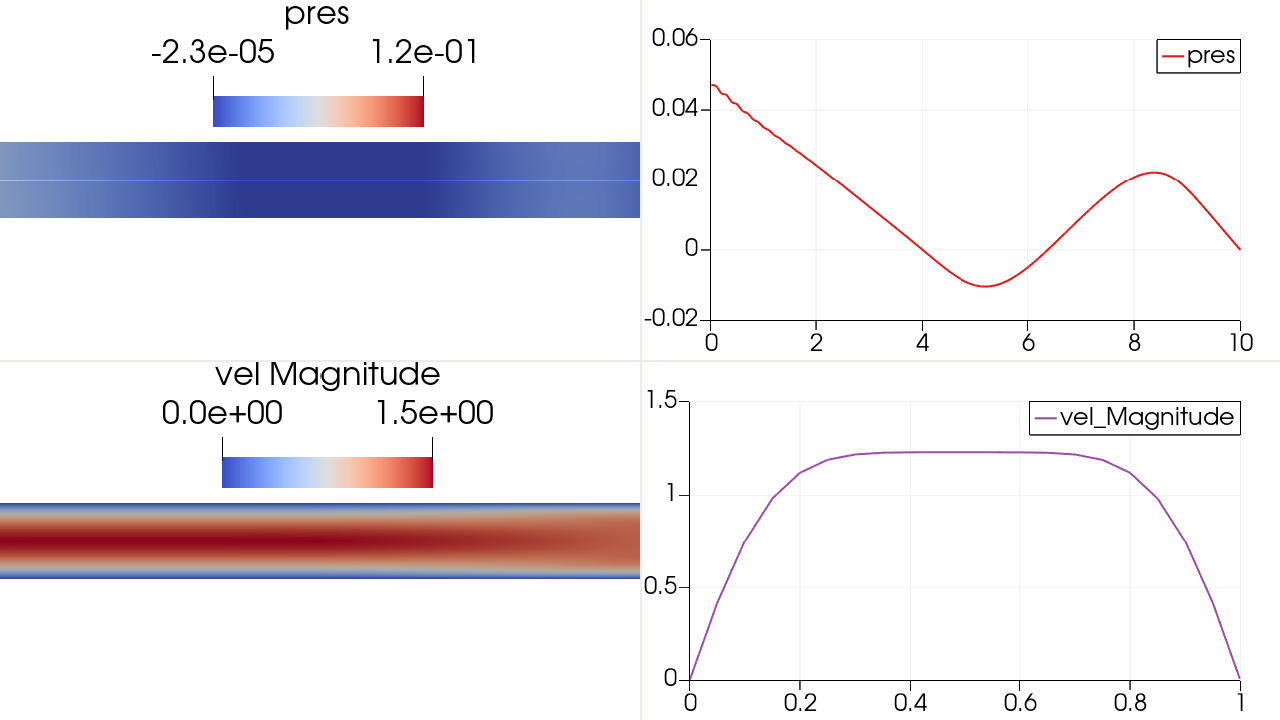
When the outlet pressure is non-zero, the solver fails to converge in general. In the below image I show the fields when p_{out} = 1, which should simply shift the pressure field above by 1. Instead, we see backflow into the domain.
p out = 1

I’m confident in the weak form, we have a similar script in Dolfin 2019 that behaves as expected, but I’m not willing to rule the weak form out as a possibility. I do think the issue lies within how I’m setting up the PETSc matrix system.
MWE
import basix
from mpi4py import MPI
import dolfinx as dfx
from dolfinx.fem.petsc import NonlinearProblem
from dolfinx.nls.petsc import NewtonSolver
from dolfinx.io import gmshio
import ufl as ufl
import matplotlib.pyplot as plt
import numpy as np
from petsc4py import PETSc

# Define boundary markers and bc function
def left(x): return np.isclose(x[0], 0.0)
def right(x): return np.isclose(x[0], 10.0)
def top(x): return np.isclose(x[1], 1.0)
def bottom(x): return np.isclose(x[1], 0.0)

def no_slip_bc(x): return np.stack((np.zeros(x.shape[1]), np.zeros(x.shape[1])))

def inlet_bc(x):
    # Parabolic
    y = x[1]
    u_max = 1.5
    profile = np.where(np.abs(y - 0.5) <= 0.5, u_max * (1 - ((y - 0.5) / 0.5) ** 2), 0.0)
    return np.stack((profile, np.zeros(x.shape[1])))

def outlet_pressure_bc(x): return np.zeros(x.shape[1])

# Define mesh
mesh = dfx.mesh.create_rectangle(MPI.COMM_WORLD, [np.array([0.0, 0.0]), np.array([10.0, 1.0])], [100, 20], dfx.mesh.CellType.triangle)

# Define mixed function space
PE = basix.ufl.element('CG', mesh.basix_cell(), degree=1)
QE = basix.ufl.element('CG', mesh.basix_cell(), degree=1, shape=(mesh.topology.dim,))
ME = basix.ufl.mixed_element([QE, PE])
W = dfx.fem.functionspace(mesh, ME)
u_sub, u_submap = W.sub(0).collapse()
p_sub, p_submap = W.sub(1).collapse()

# Define boundary conditions
fdim = mesh.topology.dim - 1
ID_left = dfx.mesh.locate_entities_boundary(mesh, fdim, left)
ID_right = dfx.mesh.locate_entities_boundary(mesh, fdim, right)
ID_top = dfx.mesh.locate_entities_boundary(mesh, fdim, top)
ID_bottom = dfx.mesh.locate_entities_boundary(mesh, fdim, bottom)

dofs_left = dfx.fem.locate_dofs_topological((W.sub(0), u_sub), fdim, ID_left)
dofs_top = dfx.fem.locate_dofs_topological((W.sub(0), u_sub), fdim, ID_top)
dofs_bottom = dfx.fem.locate_dofs_topological((W.sub(0), u_sub), fdim, ID_bottom)
dofs_right = dfx.fem.locate_dofs_topological((W.sub(0), u_sub), fdim, ID_right)
dofs_P = dfx.fem.locate_dofs_topological((W.sub(1), p_sub), fdim, ID_right)

wall = dfx.fem.Function(u_sub)
wall.interpolate(no_slip_bc)

inlet = dfx.fem.Function(u_sub)
inlet.interpolate(inlet_bc)

pressure_out = dfx.fem.Function(p_sub)
pressure_out.interpolate(outlet_pressure_bc)

bc_left = dfx.fem.dirichletbc(inlet, dofs_left, W.sub(0))
bc_top = dfx.fem.dirichletbc(wall, dofs_top, W.sub(0))
bc_bottom = dfx.fem.dirichletbc(wall, dofs_bottom, W.sub(0))
bc_P = dfx.fem.dirichletbc(pressure_out, dofs_P, W.sub(1))

bc = [bc_left, bc_top, bc_bottom, bc_P]

# Define variational problem
dt = 0.05

(v,q) = ufl.TestFunctions(W)
mu = dfx.fem.Constant(mesh, dfx.default_scalar_type(0.001))
rho = dfx.fem.Constant(mesh, dfx.default_scalar_type(1.0))
idt = dfx.fem.Constant(mesh, dfx.default_scalar_type(1.0/dt))
theta = dfx.fem.Constant(mesh, dfx.default_scalar_type(0.5))
b = dfx.fem.Constant(mesh, PETSc.ScalarType((0.0,0.0)))

W1 = dfx.fem.Function(W)
(u,p) = ufl.split(W1)

T1_1 = rho * ufl.inner(v, ufl.dot(ufl.grad(u), u)) * ufl.dx
T2_1 = mu * ufl.inner(ufl.grad(v), ufl.grad(u)) * ufl.dx
T3_1 = p * ufl.div(v) * ufl.dx
T4_1 = q * ufl.div(u) * ufl.dx
T5_1 = rho * ufl.dot(v,b) * ufl.dx
L_1  = T1_1 + T2_1 - T3_1 + T4_1 - T5_1

W0 = dfx.fem.Function(W)
(u0,p0) = ufl.split(W0)

T1_0 = rho * ufl.inner(v, ufl.dot(ufl.grad(u0), u0)) * ufl.dx
T2_0 = mu * ufl.inner(ufl.grad(v), ufl.grad(u0)) * ufl.dx
T3_0 = p * ufl.div(v) * ufl.dx
T4_0 = q * ufl.div(u0) * ufl.dx
T5_0 = rho * ufl.dot(v,b) * ufl.dx
L_0 = T1_0 + T2_0 - T3_0 + T4_0 - T5_0

F = idt * rho * ufl.inner((u-u0),v) * ufl.dx + (1.0-theta) * L_0 + theta * L_1

# SUPG/PSPG stabilization
u_norm = ufl.sqrt(ufl.inner(u0, u0))
h = ufl.CellDiameter(mesh)
tau = ( (2.0*theta*idt)**2 + (2.0*u_norm/h)**2 + (4.0*mu/h**2)**2 )**(-0.5)

residual =  idt*rho*(u - u0) + \
            theta*(rho*ufl.grad(u)*u - mu*ufl.div(ufl.grad(u)) + ufl.grad(p) - rho*b) +\
            (1.0-theta)*(rho*ufl.grad(u0)*u0 - mu*ufl.div(ufl.grad(u0)) + ufl.grad(p) - rho*b)

F_SUPG = tau * ufl.inner(ufl.grad(v)*u, residual) * ufl.dx
F_PSPG = tau * ufl.inner(ufl.grad(q), residual) * ufl.dx
F = F + F_SUPG + F_PSPG

# Define solver
problem = NonlinearProblem(F, W1, bcs=bc)
solver = NewtonSolver(MPI.COMM_WORLD, problem)
solver.convergence_criterion = "incremental"
solver.rtol = 1e-7
solver.report = True

ksp = solver.krylov_solver
opts = PETSc.Options()
option_prefix = ksp.getOptionsPrefix()
opts[f"{option_prefix}ksp_type"] = "gmres"
opts[f"{option_prefix}pc_type"] = "hypre"
ksp.setFromOptions()

t = 0
tn = 0

dfx.log.set_log_level(dfx.log.LogLevel.INFO)

vFile = dfx.io.VTKFile(MPI.COMM_WORLD, 'output/u.pvd', "w")
pFile = dfx.io.VTKFile(MPI.COMM_WORLD, 'output/p.pvd', "w")

while t < 20.0:
    n, converged = solver.solve(W1)
    print(f"Number of iterations: {n:d}")

    uf = W1.split()[0].collapse()
    pf = W1.split()[1].collapse()

    uf.name = 'vel'
    pf.name = 'pres'

    vFile.write_function(uf, tn)
    pFile.write_function(pf, tn)

    W0.x.array[:] = W1.x.array

    form = ufl.div(uf) * ufl.dx
    div = dfx.fem.assemble_scalar(dfx.fem.form(form))
    print(f"Max div: {np.abs(div)}")

    t += dt
    tn += 1

vFile.close()
pFile.close()