The mesh is way too coarse for the flow to be properly resolved.
One thing you should compare is the pressure difference and drag or lift.
Here is a code using your coarse mesh:
from mshr import *
from dolfin import *

# Create mesh
channel = Rectangle(Point(0, 0), Point(2.2, 0.41))
cylinder = Circle(Point(0.2, 0.2), 0.05)
domain = channel - cylinder
mesh = generate_mesh(domain, 64)


with XDMFFile("mesh.xdmf") as xdmf:
    xdmf.write(mesh)
Using in with the code from the dolfinx tutorial (no modifications to the splitting scheme, only to reading in the mesh), yields
# # Test problem 2: Flow past a cylinder (DFG 2D-3 benchmark)
#
# Author: Jørgen S. Dokken
#
# In this section, we will turn our attention to a slightly more challenging problem: flow past a cylinder. The geometry and parameters are taken from the [DFG 2D-3 benchmark](https://www.featflow.de/en/benchmarks/cfdbenchmarking/flow/dfg_benchmark3_re100.html) in FeatFlow.
#
# To be able to solve this problem efficiently and ensure numerical stability, we will substitute our first order backward difference scheme with a Crank-Nicholson discretization in time, and a semi-implicit Adams-Bashforth approximation of the non-linear term.
#
# ```{admonition} Computationally demanding demo
# This demo is computationally demanding, with a run-time up to 15 minutes, as it is using parameters from the DFG 2D-3 benchmark, which consists of 12800 time steps. It is adviced to download this demo and not run it in a browser. This runtime of the demo can be increased by using 2 or 3 mpi processes.
# ```
#
# The computational geometry we would like to use is
# 
#
# The kinematic velocity is given by $\nu=0.001=\frac{\mu}{\rho}$ and the inflow velocity profile is specified as
#
# $$
# u(x,y,t) = \left( \frac{4Uy(0.41-y)}{0.41^2}, 0 \right)
# $$
#
# $$
# U=U(t) = 1.5\sin(\pi t/8)
# $$
#
# which has a maximum magnitude of $1.5$ at $y=0.41/2$. We do not use any scaling for this problem since all exact parameters are known.
#
# ## Mesh generation
#
# As in the [Deflection of a membrane](./../chapter1/membrane_code.ipynb) we use GMSH to generate the mesh. We fist create the rectangle and obstacle.
#
# +
import os
import numpy as np
import matplotlib.pyplot as plt
import tqdm.autonotebook
from mpi4py import MPI
from petsc4py import PETSc
from basix.ufl import element
from dolfinx.fem import (
Constant,
Function,
functionspace,
assemble_scalar,
dirichletbc,
form,
locate_dofs_topological,
set_bc,
)
from dolfinx.fem.petsc import (
apply_lifting,
assemble_matrix,
assemble_vector,
create_vector,
create_matrix,
set_bc,
)
from dolfinx.mesh import exterior_facet_indices, locate_entities_boundary, meshtags
from dolfinx.geometry import bb_tree, compute_collisions_points, compute_colliding_cells
from dolfinx.io import VTXWriter, XDMFFile
from ufl import (
FacetNormal,
Measure,
TestFunction,
TrialFunction,
as_vector,
div,
dot,
dx,
inner,
lhs,
grad,
nabla_grad,
rhs,
)
with XDMFFile(MPI.COMM_WORLD, "mesh.xdmf", "r") as xdmf:
mesh = xdmf.read_mesh(name="mesh")
gdim = mesh.geometry.dim
fdim = mesh.topology.dim - 1
mesh.topology.create_connectivity(fdim, fdim + 1)
num_facets = (
mesh.topology.index_map(fdim).size_local + mesh.topology.index_map(fdim).num_ghosts
)
inlet_marker, outlet_marker, wall_marker, obstacle_marker = 2, 3, 4, 5
facets = np.arange(num_facets, dtype=np.int32)
values = np.zeros_like(facets)
values[exterior_facet_indices(mesh.topology)] = obstacle_marker
values[locate_entities_boundary(mesh, fdim, lambda x: np.isclose(x[0], 0))] = (
inlet_marker
)
values[locate_entities_boundary(mesh, fdim, lambda x: np.isclose(x[0], 2.2))] = (
outlet_marker
)
values[
locate_entities_boundary(
mesh, fdim, lambda x: np.isclose(x[1], 0) | np.isclose(x[1], 0.41)
)
] = wall_marker
ft = meshtags(mesh, fdim, facets, values)
t = 0
T = 8 # Final time
dt = 1 / 1600 # Time step size
num_steps = int(T / dt)
k = Constant(mesh, PETSc.ScalarType(dt))
mu = Constant(mesh, PETSc.ScalarType(0.001)) # Dynamic viscosity
rho = Constant(mesh, PETSc.ScalarType(1)) # Density
# ```{admonition} Reduced end-time of problem
# In the current demo, we have reduced the run time to one second to make it easier to illustrate the concepts of the benchmark. By increasing the end-time `T` to 8, the runtime in a notebook is approximately 25 minutes. If you convert the notebook to a python file and use `mpirun`, you can reduce the runtime of the problem.
# ```
#
# ## Boundary conditions
#
# As we have created the mesh and relevant mesh tags, we can now specify the function spaces `V` and `Q` along with the boundary conditions. As the `ft` contains markers for facets, we use this class to find the facets for the inlet and walls.
#
# +
v_cg2 = element("Lagrange", mesh.topology.cell_name(), 2, shape=(mesh.geometry.dim,))
s_cg1 = element("Lagrange", mesh.topology.cell_name(), 1)
V = functionspace(mesh, v_cg2)
Q = functionspace(mesh, s_cg1)
fdim = mesh.topology.dim - 1
# Define boundary conditions
class InletVelocity:
def __init__(self, t):
self.t = t
def __call__(self, x):
values = np.zeros((gdim, x.shape[1]), dtype=PETSc.ScalarType)
values[0] = (
4 * 1.5 * np.sin(self.t * np.pi / 8) * x[1] * (0.41 - x[1]) / (0.41**2)
)
return values
# Inlet
u_inlet = Function(V)
inlet_velocity = InletVelocity(t)
u_inlet.interpolate(inlet_velocity)
bcu_inflow = dirichletbc(
u_inlet, locate_dofs_topological(V, fdim, ft.find(inlet_marker))
)
# Walls
u_nonslip = np.array((0,) * mesh.geometry.dim, dtype=PETSc.ScalarType)
bcu_walls = dirichletbc(
u_nonslip, locate_dofs_topological(V, fdim, ft.find(wall_marker)), V
)
# Obstacle
bcu_obstacle = dirichletbc(
u_nonslip, locate_dofs_topological(V, fdim, ft.find(obstacle_marker)), V
)
bcu = [bcu_inflow, bcu_obstacle, bcu_walls]
# Outlet
bcp_outlet = dirichletbc(
PETSc.ScalarType(0), locate_dofs_topological(Q, fdim, ft.find(outlet_marker)), Q
)
bcp = [bcp_outlet]
# -
# ## Variational form
#
# As opposed to [Pouseille flow](./ns_code1.ipynb), we will use a Crank-Nicolson discretization, and an semi-implicit Adams-Bashforth approximation.
# The first step can be written as
#
# $$
# \rho\left(\frac{u^*- u^n}{\delta t} + \left(\frac{3}{2}u^{n} - \frac{1}{2} u^{n-1}\right)\cdot \frac{1}{2}\nabla (u^*+u^n) \right) - \frac{1}{2}\mu \Delta( u^*+ u^n )+ \nabla p^{n-1/2} = f^{n+\frac{1}{2}} \qquad \text{ in } \Omega
# $$
#
# $$
# u^{*}=g(\cdot, t^{n+1}) \qquad \text{ on } \partial \Omega_{D}
# $$
#
# $$
# \frac{1}{2}\nu \nabla (u^*+u^n) \cdot n = p^{n-\frac{1}{2}} \qquad \text{ on } \partial \Omega_{N}
# $$
#
# where we have used the two previous time steps in the temporal derivative for the velocity, and compute the pressure staggered in time, at the time between the previous and current solution. The second step becomes
#
# $$
# \nabla \phi = -\frac{\rho}{\delta t} \nabla \cdot u^* \qquad\text{in } \Omega,
# $$
#
# $$
# \nabla \phi \cdot n = 0 \qquad \text{on } \partial \Omega_D,
# $$
#
# $$
# \phi = 0 \qquad\text{on } \partial\Omega_N
# $$
#
# where $p^{n+\frac{1}{2}}=p^{n-\frac{1}{2}} + \phi$.
# Finally, the third step is
#
# $$
# \rho (u^{n+1}-u^{*}) = -\delta t \nabla\phi.
# $$
#
# We start by defining all the variables used in the variational formulations.
#
u = TrialFunction(V)
v = TestFunction(V)
u_ = Function(V)
u_.name = "u"
u_s = Function(V)
u_n = Function(V)
u_n1 = Function(V)
p = TrialFunction(Q)
q = TestFunction(Q)
p_ = Function(Q)
p_.name = "p"
phi = Function(Q)
# Next, we define the variational formulation for the first step, where we have integrated the diffusion term, as well as the pressure term by parts.
#
f = Constant(mesh, PETSc.ScalarType((0, 0)))
F1 = rho / k * dot(u - u_n, v) * dx
F1 += inner(dot(1.5 * u_n - 0.5 * u_n1, 0.5 * nabla_grad(u + u_n)), v) * dx
F1 += 0.5 * mu * inner(grad(u + u_n), grad(v)) * dx - dot(p_, div(v)) * dx
F1 += dot(f, v) * dx
a1 = form(lhs(F1))
L1 = form(rhs(F1))
A1 = create_matrix(a1)
b1 = create_vector(L1)
# Next we define the second step
#
a2 = form(dot(grad(p), grad(q)) * dx)
L2 = form(-rho / k * dot(div(u_s), q) * dx)
A2 = assemble_matrix(a2, bcs=bcp)
A2.assemble()
b2 = create_vector(L2)
# We finally create the last step
#
a3 = form(rho * dot(u, v) * dx)
L3 = form(rho * dot(u_s, v) * dx - k * dot(nabla_grad(phi), v) * dx)
A3 = assemble_matrix(a3)
A3.assemble()
b3 = create_vector(L3)
# As in the previous tutorials, we use PETSc as a linear algebra backend.
#
# +
# Solver for step 1
solver1 = PETSc.KSP().create(mesh.comm)
solver1.setOperators(A1)
solver1.setType(PETSc.KSP.Type.BCGS)
pc1 = solver1.getPC()
pc1.setType(PETSc.PC.Type.JACOBI)
# Solver for step 2
solver2 = PETSc.KSP().create(mesh.comm)
solver2.setOperators(A2)
solver2.setType(PETSc.KSP.Type.MINRES)
pc2 = solver2.getPC()
pc2.setType(PETSc.PC.Type.HYPRE)
pc2.setHYPREType("boomeramg")
# Solver for step 3
solver3 = PETSc.KSP().create(mesh.comm)
solver3.setOperators(A3)
solver3.setType(PETSc.KSP.Type.CG)
pc3 = solver3.getPC()
pc3.setType(PETSc.PC.Type.SOR)
# -
# ## Verification of the implementation compute known physical quantities
#
# As a further verification of our implementation, we compute the drag and lift coefficients over the obstacle, defined as
#
# $$
# C_{\text{D}}(u,p,t,\partial\Omega_S) = \frac{2}{\rho L U_{mean}^2}\int_{\partial\Omega_S}\rho \nu n \cdot \nabla u_{t_S}(t)n_y -p(t)n_x~\mathrm{d} s,
# $$
#
# $$
# C_{\text{L}}(u,p,t,\partial\Omega_S) = -\frac{2}{\rho L U_{mean}^2}\int_{\partial\Omega_S}\rho \nu n \cdot \nabla u_{t_S}(t)n_x + p(t)n_y~\mathrm{d} s,
# $$
#
# where $u_{t_S}$ is the tangential velocity component at the interface of the obstacle $\partial\Omega_S$, defined as $u_{t_S}=u\cdot (n_y,-n_x)$, $U_{mean}=1$ the average inflow velocity, and $L$ the length of the channel. We use `UFL` to create the relevant integrals, and assemble them at each time step.
#
n = -FacetNormal(mesh) # Normal pointing out of obstacle
dObs = Measure("ds", domain=mesh, subdomain_data=ft, subdomain_id=obstacle_marker)
u_t = inner(as_vector((n[1], -n[0])), u_)
drag = form(2 / 0.1 * (mu / rho * inner(grad(u_t), n) * n[1] - p_ * n[0]) * dObs)
lift = form(-2 / 0.1 * (mu / rho * inner(grad(u_t), n) * n[0] + p_ * n[1]) * dObs)
if mesh.comm.rank == 0:
C_D = np.zeros(num_steps, dtype=PETSc.ScalarType)
C_L = np.zeros(num_steps, dtype=PETSc.ScalarType)
t_u = np.zeros(num_steps, dtype=np.float64)
t_p = np.zeros(num_steps, dtype=np.float64)
# We will also evaluate the pressure at two points, one in front of the obstacle, $(0.15, 0.2)$, and one behind the obstacle, $(0.25, 0.2)$. To do this, we have to find which cell contains each of the points, so that we can create a linear combination of the local basis functions and coefficients.
#
tree = bb_tree(mesh, mesh.geometry.dim)
points = np.array([[0.15, 0.2, 0], [0.25, 0.2, 0]])
cell_candidates = compute_collisions_points(tree, points)
colliding_cells = compute_colliding_cells(mesh, cell_candidates, points)
front_cells = colliding_cells.links(0)
back_cells = colliding_cells.links(1)
if mesh.comm.rank == 0:
p_diff = np.zeros(num_steps, dtype=PETSc.ScalarType)
# ## Solving the time-dependent problem
#
# ```{admonition} Stability of the Navier-Stokes equation
# Note that the current splitting scheme has to fullfil the a [Courant–Friedrichs–Lewy condition](https://en.wikipedia.org/wiki/Courant%E2%80%93Friedrichs%E2%80%93Lewy_condition). This limits the spatial discretization with respect to the inlet velocity and temporal discretization.
# Other temporal discretization schemes such as the second order backward difference discretization or Crank-Nicholson discretization with Adams-Bashforth linearization are better behaved than our simple backward difference scheme.
# ```
#
# As in the previous example, we create output files for the velocity and pressure and solve the time-dependent problem. As we are solving a time dependent problem with many time steps, we use the `tqdm`-package to visualize the progress. This package can be installed with `pip3`.
#
from pathlib import Path
folder = Path("results")
folder.mkdir(exist_ok=True, parents=True)
vtx_u = VTXWriter(mesh.comm, "dfg2D-3-u.bp", [u_], engine="BP4")
vtx_p = VTXWriter(mesh.comm, "dfg2D-3-p.bp", [p_], engine="BP4")
vtx_u.write(t)
vtx_p.write(t)
progress = tqdm.autonotebook.tqdm(desc="Solving PDE", total=num_steps)
for i in range(num_steps):
progress.update(1)
# Update current time step
t += dt
# Update inlet velocity
inlet_velocity.t = t
u_inlet.interpolate(inlet_velocity)
# Step 1: Tentative velocity step
A1.zeroEntries()
assemble_matrix(A1, a1, bcs=bcu)
A1.assemble()
with b1.localForm() as loc:
loc.set(0)
assemble_vector(b1, L1)
apply_lifting(b1, [a1], [bcu])
b1.ghostUpdate(addv=PETSc.InsertMode.ADD_VALUES, mode=PETSc.ScatterMode.REVERSE)
set_bc(b1, bcu)
solver1.solve(b1, u_s.vector)
u_s.x.scatter_forward()
# Step 2: Pressure corrrection step
with b2.localForm() as loc:
loc.set(0)
assemble_vector(b2, L2)
apply_lifting(b2, [a2], [bcp])
b2.ghostUpdate(addv=PETSc.InsertMode.ADD_VALUES, mode=PETSc.ScatterMode.REVERSE)
set_bc(b2, bcp)
solver2.solve(b2, phi.vector)
phi.x.scatter_forward()
p_.vector.axpy(1, phi.vector)
p_.x.scatter_forward()
# Step 3: Velocity correction step
with b3.localForm() as loc:
loc.set(0)
assemble_vector(b3, L3)
b3.ghostUpdate(addv=PETSc.InsertMode.ADD_VALUES, mode=PETSc.ScatterMode.REVERSE)
solver3.solve(b3, u_.vector)
u_.x.scatter_forward()
# Write solutions to file
vtx_u.write(t)
vtx_p.write(t)
# Update variable with solution form this time step
with u_.vector.localForm() as loc_, u_n.vector.localForm() as loc_n, u_n1.vector.localForm() as loc_n1:
loc_n.copy(loc_n1)
loc_.copy(loc_n)
# Compute physical quantities
# For this to work in paralell, we gather contributions from all processors
# to processor zero and sum the contributions.
drag_coeff = mesh.comm.gather(assemble_scalar(drag), root=0)
lift_coeff = mesh.comm.gather(assemble_scalar(lift), root=0)
p_front = None
if len(front_cells) > 0:
p_front = p_.eval(points[0], front_cells[:1])
p_front = mesh.comm.gather(p_front, root=0)
p_back = None
if len(back_cells) > 0:
p_back = p_.eval(points[1], back_cells[:1])
p_back = mesh.comm.gather(p_back, root=0)
if mesh.comm.rank == 0:
t_u[i] = t
t_p[i] = t - dt / 2
C_D[i] = sum(drag_coeff)
C_L[i] = sum(lift_coeff)
# Choose first pressure that is found from the different processors
for pressure in p_front:
if pressure is not None:
p_diff[i] = pressure[0]
break
for pressure in p_back:
if pressure is not None:
p_diff[i] -= pressure[0]
break
vtx_u.close()
vtx_p.close()
# ## Verification using data from FEATFLOW
#
# As FEATFLOW has provided data for different discretization levels, we compare our numerical data with the data provided using `matplotlib`.
#
if mesh.comm.rank == 0:
if not os.path.exists("figures"):
os.mkdir("figures")
num_velocity_dofs = V.dofmap.index_map_bs * V.dofmap.index_map.size_global
num_pressure_dofs = Q.dofmap.index_map_bs * V.dofmap.index_map.size_global
turek = np.loadtxt("bdforces_lv4")
turek_p = np.loadtxt("pointvalues_lv4")
fig = plt.figure(figsize=(25, 8))
l1 = plt.plot(
t_u,
C_D,
label=r"FEniCSx ({0:d} dofs)".format(num_velocity_dofs + num_pressure_dofs),
linewidth=2,
)
l2 = plt.plot(
turek[1:, 1],
turek[1:, 3],
marker="x",
markevery=50,
linestyle="",
markersize=4,
label="FEATFLOW (42016 dofs)",
)
plt.title("Drag coefficient")
plt.grid()
plt.legend()
plt.savefig("figures/drag_comparison.png")
fig = plt.figure(figsize=(25, 8))
l1 = plt.plot(
t_u,
C_L,
label=r"FEniCSx ({0:d} dofs)".format(num_velocity_dofs + num_pressure_dofs),
linewidth=2,
)
l2 = plt.plot(
turek[1:, 1],
turek[1:, 4],
marker="x",
markevery=50,
linestyle="",
markersize=4,
label="FEATFLOW (42016 dofs)",
)
plt.title("Lift coefficient")
plt.grid()
plt.legend()
plt.savefig("figures/lift_comparison.png")
fig = plt.figure(figsize=(25, 8))
l1 = plt.plot(
t_p,
p_diff,
label=r"FEniCSx ({0:d} dofs)".format(num_velocity_dofs + num_pressure_dofs),
linewidth=2,
)
l2 = plt.plot(
turek[1:, 1],
turek_p[1:, 6] - turek_p[1:, -1],
marker="x",
markevery=50,
linestyle="",
markersize=4,
label="FEATFLOW (42016 dofs)",
)
plt.title("Pressure difference")
plt.grid()
plt.legend()
plt.savefig("figures/pressure_comparison.png")
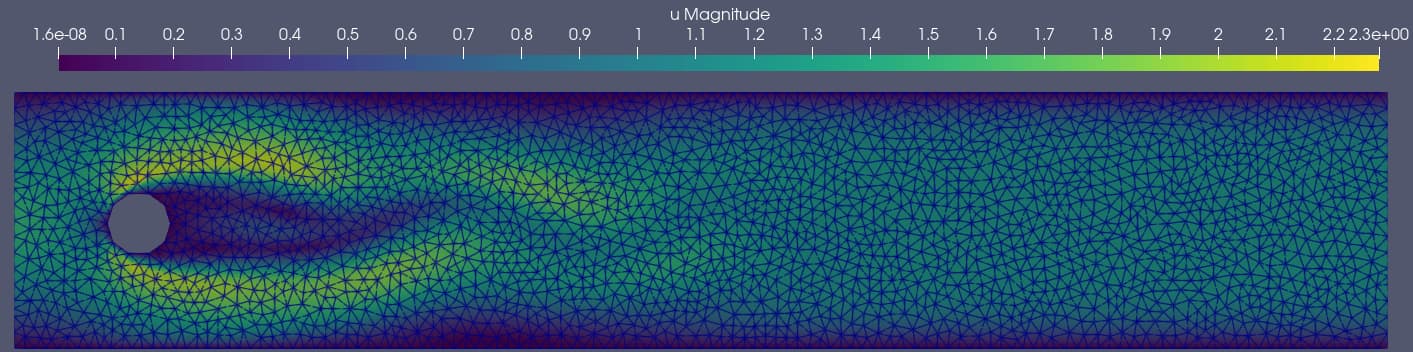
with the following flow (at the end time T=8):
and comparisons
Indicating that the mesh is too coarse.
I am not going to debug your full code to find the differences.
Using a constant inflow profile, as in the old tutorial,changing T=5
and the inlet profile to
class InletVelocity:
    def __init__(self, t):
        self.t = t

    def __call__(self, x):
        values = np.zeros((gdim, x.shape[1]), dtype=PETSc.ScalarType)
        values[0] = 4 * 1.5 * x[1] * (0.41 - x[1]) / (0.41**2)
        return values
yields
at time equal to 1, so I think you have done something wrong in your implementation.