Poisson equation with Dirichlet condition on internal point

mekong · September 24, 2025, 3:01pm

Dear all,
Consider the Poisson equation \frac{d^2 u}{dx^2} = f on a line x \in [0,1]. I want to solve this equation by imposing one Dirichlet BC on the left edge x=0, and by fixing the value of the field u to u_0 on the middle point in the mesh x=1/2.

How can I achieve this? This post did not help. Also, I tried adding a penalty term

F_N = alpha/r_mesh * \
    ((u('+') - u0('+')) * nu_u('+') + \
     (u('-') - u0('-')) * nu_u('-')) * ds_m

where ds_m is the domain relative to the middle vertex, defined as

# read the vertices
vf = msh.read_mesh_components(lmsh.mesh, lmsh.mesh.topology().dim() - 1, io.add_trailing_slash(rarg.args.input_directory) + "vertex_mesh.h5", "vf")
ds_m = Measure("dS", domain=lmsh.mesh, subdomain_data=vf, subdomain_id=3)

or to a Dirichlet condition on the ds_m as

bc_u_m = DirichletBC(fsp.Q, fsp.u_exact, rmsh.vf, 3)

In both cases, the solver diverges.

Any ideas ? Thank you

dokken · September 24, 2025, 4:41pm

Please provide a minimal reproducible example. With only snippets of your code, it’s had to say why the solver diverges.

mekong · September 24, 2025, 9:33pm

Sure, here is a minimal worked example which I produced for you.
The example reads the mesh files line_mesh.h5 and vertex_mesh.h5, note that I need this read from file to incorporate the minimal working example in the original code.
Please download the two .h5 files from here, which you should put in `path_of_solve_dot_py/mesh_files’.

The code which solves the Poisson equation, solve.py, is

from fenics import *
import numpy as np
import ufl
import sys

mesh_path = 'mesh_files/'


mesh = Mesh()
with HDF5File(mesh.mpi_comm(), mesh_path + "line_mesh.h5", "r") as infile:
    infile.read(mesh, 'mesh', False)


# read lines and vertices
cf = MeshFunction("size_t", mesh, mesh.topology().dim())
with HDF5File(mesh.mpi_comm(), mesh_path + "line_mesh.h5", "r") as infile:
    infile.read(cf, 'cf')
    
vf = MeshFunction("size_t", mesh, mesh.topology().dim()-1)
with HDF5File(mesh.mpi_comm(), mesh_path + "vertex_mesh.h5", "r") as infile:
    infile.read(vf, 'vf')




# radius of the smallest cell in the mesh
r_mesh = mesh.hmin()

# measures for the line, for left and right points and for middle point
dx = Measure("dx", domain=mesh, subdomain_data=cf, subdomain_id=1)
ds_l = Measure("ds", domain=mesh, subdomain_data=vf, subdomain_id=2)
ds_r = Measure("ds", domain=mesh, subdomain_data=vf, subdomain_id=3)
ds_m = Measure("dS", domain=mesh, subdomain_data=vf, subdomain_id=4)
ds_lr = Measure("ds", domain=mesh)


# define boundaries for left and right points, and for middle point
boundary = 'on_boundary'
boundary_l = f'near(x[0], {0.0})'
boundary_r = f'near(x[0], {1.0})'
boundary_m = f'near(x[0], {0.5})'

Q = FunctionSpace(mesh, 'P', 4)

u = Function(Q)
nu_u = TestFunction(Q)
f = Function(Q)
J_u = TrialFunction(Q)
u_exact = Function(Q)


# consider a Poisson equation for which I know the exact solution
class u_exact_expression(UserExpression):
    def eval(self, values, x):
        # test case 1
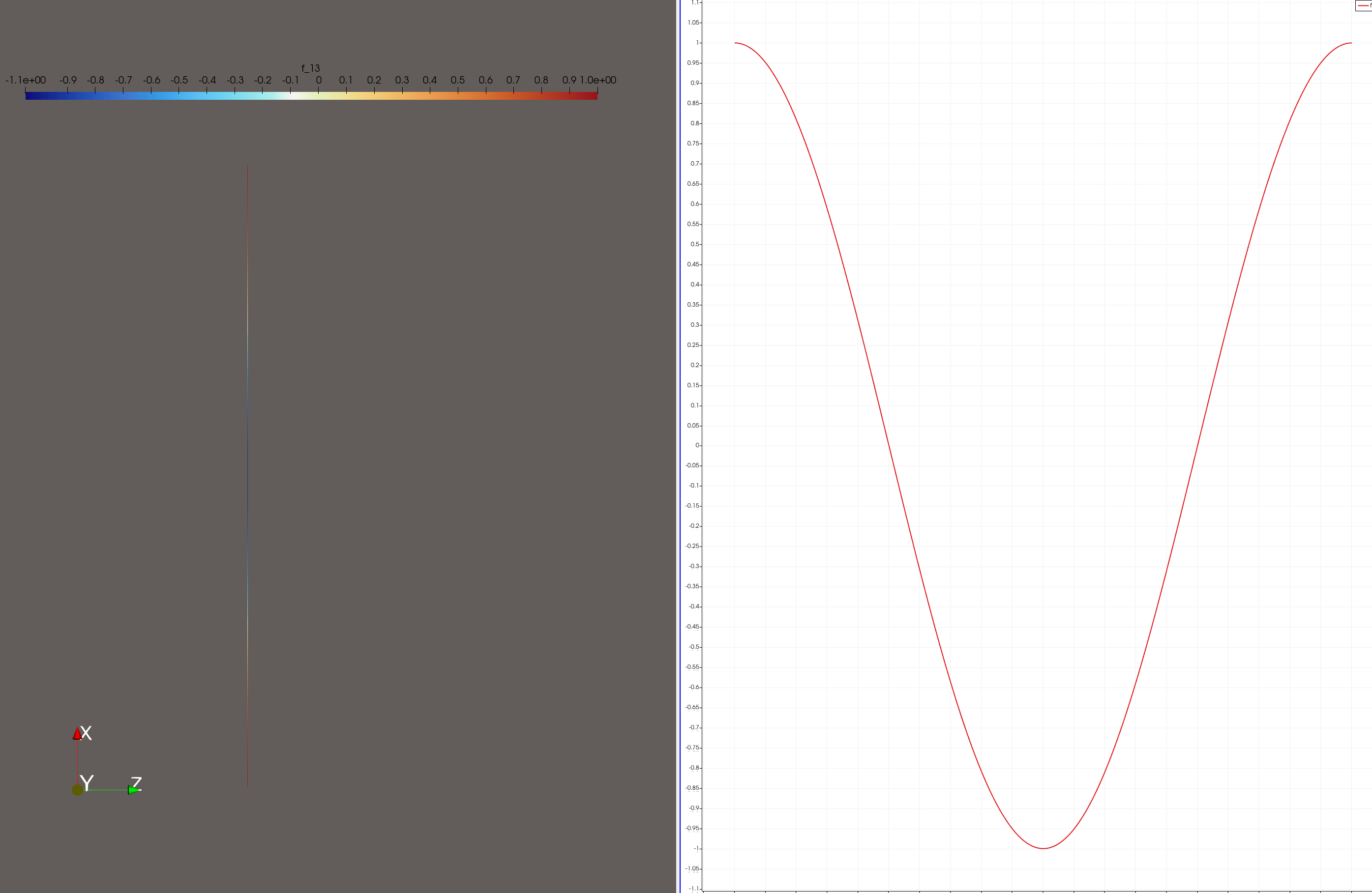
        values[0] = np.cos(2 * np.pi * x[0]) 

    def value_shape(self):
        return (1,)


class grad_u_expression(UserExpression):
    def eval(self, values, x):
        # test case 1
        values[0] = - 2 * np.pi / 1 * np.sin(2 * np.pi * x[0]) 

    def value_shape(self):
        return (1,)


class laplacian_u_expression(UserExpression):
    def eval(self, values, x):
        # test case 1
        values[0] = -( 2 * np.pi )**2 * np.cos(2 * np.pi * x[0]) 
          
    def value_shape(self):
        return (1,)


u_exact.interpolate(u_exact_expression(element=Q.ufl_element()))
f.interpolate(laplacian_u_expression(element=Q.ufl_element()))


# Dirichlet boundary conditions on left and right edge
bc_l = DirichletBC(Q, u_exact, boundary_l )
bc_r = DirichletBC(Q, u_exact, boundary_r )

# tentative condition to enforce u = u _exact at the middle (m) point
bc_m = DirichletBC(Q, u_exact, boundary_m )

#case A: this works
bcs = [bc_l, bc_r]
# case B: this does not work
# bcs = [bc_l, bc_m]

i = ufl.indices(1)
facet_normal = FacetNormal(mesh)


# variational problem
F = (u.dx(i) * nu_u.dx(i) + f * nu_u) * dx \
    - facet_normal[i] * (u.dx(i)) * nu_u * ds_lr



J = derivative(F, u, J_u)
problem = NonlinearVariationalProblem(F, u, bcs, J)
solver = NonlinearVariationalSolver(problem)

# set the solver parameters here
params = {'nonlinear_solver': 'newton',
          'newton_solver':
              {
                  'linear_solver': 'superlu',
                  'absolute_tolerance': 1e-12,
                  'relative_tolerance': 1e-12,
                  'maximum_iterations': 1000000,
                  'relaxation_parameter': 0.95,
              }
          }
solver.parameters.update(params)

solver.solve()

print(f'\nerror = {assemble((u - u_exact)**2 * dx)/assemble(Constant(1)* dx)}')

If you run it by adding BCs on the left and right edge (case A in solve.py) bcs = [bc_l, bc_r] it works:

e# python3 solve.py 
Solving nonlinear variational problem.
  Newton iteration 0: r (abs) = 1.144e+04 (tol = 1.000e-12) r (rel) = 1.000e+00 (tol = 1.000e-12)
[...] 
 Newton iteration 10: r (abs) = 1.118e-09 (tol = 1.000e-12) r (rel) = 9.768e-14 (tol = 1.000e-12)
  Newton solver finished in 10 iterations and 10 linear solver iterations.

error = 4.8274638233736306e-27

if you run it by adding a Dirichlet BC on the left edge and a Dirichlet condition on the middle edge with bcs = [bc_l, bc_m] (case B), it fails:

# python3 solve.py 
Solving nonlinear variational problem.
  Newton iteration 0: r (abs) = 1.402e+04 (tol = 1.000e-12) r (rel) = 1.000e+00 (tol = 1.000e-12)
  [...]
  Newton iteration 11: r (abs) = 8.500e-09 (tol = 1.000e-12) r (rel) = 6.065e-13 (tol = 1.000e-12)
  Newton solver finished in 11 iterations and 11 linear solver iterations.

error = 1367.2355166035707

Thank you for your help.

dokken · September 25, 2025, 2:03pm

First of all, as your mesh is just a line, why cant you just use a UnitIntervalMesh for the reproducible example?

Secondly, if your exact solution on the unit interval is
u=\cos(2\pi x), then \nabla u=-2\pi\sin(2 \pi x) which is equal to zero at the boundaries.
In your variational form, you have kept the term

which is what makes your solution wrong.
If you remove this term, you get the correct behavior.

Finally, why are you damping the non-linear solver?
Since the problem is linear, using a damping-factor of 1.0 will allow it to solve the problem in one iteration.
You should also try to visualize your solution, as it clearly shows the issue:

After removing the aforementioned term:

mekong · September 25, 2025, 8:25pm

Hello,
I am deliberately not using UnitIntervalMesh because later on I would like to tag the mid point as a dS and impose this same constraint on the midpoint a a penalty.

Here the exact solution is used as a benchmark to check if the ODE solution is correct, but in general I want to solve an ODE by fixing the value of the unknown u at the left edge and at the midpoint, and I don’t know that the gradient of the solution vanishes at the boundaries.

So, given the problem
d^2 u /dx^2 = f for x \in (0,1)
with u(0) = a and u(1/2) = b,
I don’t see what reasoning would imply that the term facet_normal[i] * (u.dx(i)) * nu_u * ds_lr must be set to zero.

That is a leftover of a code which I used for nonlinear problems.

dokken · September 25, 2025, 8:46pm

If you want it to match the exact solution, that is the Neumann boundary condition at the interface.
As you can see, if you do not impose the Neumann condition, you get another solution, where du/dn!=0 at x=1

But for anyone trying to reproduce your issue, adding files on Dropbox that might disappear in the future is not the easiest way to get help.

mekong · September 25, 2025, 8:56pm

This means that fixing u at x=0 (with a Dirichlet boundary condition) and x=1/2 (with an
“interior” condition) does not uniquely determine the solution. Is this known on a rigorous level ?

You are right, I will do without mesh files in the future.

dokken · September 26, 2025, 5:27am

Yours are uniquely determining the solution form 0 to 0.5 (as you can see above).
It is of course clear that on the interval 0.5 to 1, you would get to different solutions if you include the boundary term or not, as it alters the discrete system.

Leaving the term applies a strange boundary condition at x=1.
You can see this without you subdivision by solving the Poisson equation on an interval, where you fix the bcs at x=0, and choose to include or ignore the flux term at x=1

mekong · September 30, 2025, 12:17pm

That makes perfect sense, thank you. I have a related question about this, but I believe it deserves a different post. I will make one.

dparsons · September 30, 2025, 1:06pm

What I learnt from this topic is that DirichletBC can be applied just as easily to internal boundaries as external. I had always thought it applied strictly only to external boundaries, and any internal condition would have to be enforced weakly. Useful to know that internal conditions can also be imposed strongly via DirichletBC. Thank you both for the discussion.

dokken · October 1, 2025, 1:13pm

The mathematical setting for applying strong Dirichlet conditions on a linear system is explained in detail in:

which tries to show that the spatial position of a dof doesn’t matter.

dparsons · October 1, 2025, 2:10pm

To be honest, that tutorial doesn’t make it obvious that the procedure also applies to internal dofs.

It refers to ∂Ω, which I would read as an external boundary, and collects facets for the dofs using exterior_facet_indices. But from the discussion here I am now informed that it also works with internal dofs.

dokken · October 1, 2025, 3:00pm

In the tutorial, I separate it into being constrained and unconstrained degrees of freedom (which doesn’t really have any notion of boundary or not). Of course the example uses the exterior boundary.

I might add a note that mentions this explicitly.

dparsons · October 1, 2025, 3:56pm

Could be useful to mention it explicitly. It’s kind of a question of conceptualisation of how to solve a problem. For my own work, I think in terms of the boundaries and the physics at those boundaries. So for me the degrees of freedom are a technical numerical implementation detail which I try not to think about more than I need to (I like FEniCS for the way that ufl lets me implement the mathematics of the weak formulation directly, minimising the amount of numerical technical details that I need to think about). This example gives me a case where I need to think about them more carefully.

When I get time I might set up a simple 2d example showing where I might use an internal Dirichlet bc.

Topic		Replies	Views
Simple Poisson equation in 1D with von Neumann condition on the left variational formulation	4	2045	January 8, 2020
Von Neumann boundary condition on internal boundary not working mesh	1	980	February 14, 2019
Set Internal Boundary Condition Using Mixed Dimensional Space variational formulation	5	1776	April 10, 2020
Solving a Poisson type equation variational formulation	1	521	January 15, 2020
3D Poisson - problem with neumann BC variational formulation	6	1157	August 12, 2020

Poisson equation with Dirichlet condition on internal point

Related topics