Problem with the solution close to the border [Overshoots close to Dirichlet Boundary Condition]

[MortezaAram]

Hi everybody,

I’ve recently started working with Fenics and I have a problem with the final solution which is a distribution of temperature in the steady-state case; That is, when we don’t have any temporal variation and the system has reached an equilibrium. The problem is that I notice a wild oscillation throughout the border where I forced the temperature to remain 20 degrees C by using Outer_bc = DirichletBC(V, 20, DomainBoundary()). I did a simple simulation for a cylinder where I expect to see a pretty uniform distribution of 37 degrees C in the middle and a gradual decrease to 20 C towards the border which has a fixed temperature (please see the snippet of my code for this scenario).

First I had used a 1st order CG for the function space, so I suspected the problem might have come from poor meshing. So I changed the function space to 2nd order CG and it seemed to solve the problem (please see the attached temperature profiles of the two simulations). I was happy and I thought the problem would completely disappear as I kept increasing the resolution by importing a finer and finer mesh. So I decided to make my mesh even finer to get a smoother profile and I didn’t expect to see the old problem resurface. But to my consternation, it did. I increased the number of mesh elements from 400K to almost 4 million and sure I ran out of memory when I tried to run the code in series. So I ran it in parallel and in the final result I got very good and smooth distribution in the middle but those overshoots to 55 degrees C and even higher came back around the edges!

Is this a problem of meshing really or am I missing something here? To me, it doesn’t seem to come from just poor meshing because it happened even for a very fine mesh at the end, but why didn’t it happen for the 2nd run when I just used the old (coarser) mesh with just increased degrees of freedom (2nd order CG)??

I’m wondering if someone has experienced the same problem. It’s highly appreciated if you share your thought and experiences in this regard and many thanks in advance.

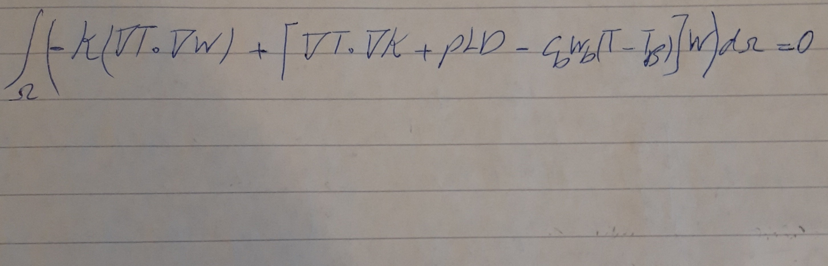
from fenics import *

#%% Declaration of Constants
Kapa_value = [0.5, 0.55] #Thermal Conductivity (W/m/'c), [Muscle, Tumor] 
Cp_value = [3421, 3500]#Heat Capacity (J/Kg/'c), [Muscle, Tumor]
Cb = 3617 #specific heat (Heat Capacity) of blood (J/Kg/'c)
Wb_value = [0.8, 0.5] #local perfusion rate (kg/m3/s), [Muscle, Tumor]
Tb = 37   #Arterial blood temperature
Rho_value = [1090, 1040]#Density of Muscle (Kg/m3)
Bolus_Temp = Constant(20)
Body_Temp = Constant(37) #Normal body temperature

#%% Classic Mesh conversion using dolfin-convert (legacy)!
mesh = Mesh('../GeoMesh.xml') 
Markers = MeshFunction('size_t',mesh,'../GeoMesh_physical_region.xml')
BCs = MeshFunction('size_t',mesh,'../GeoMesh_facet_region.xml')
dx = Measure('dx', domain=mesh, subdomain_data=Markers)

#%% Subdomains' property assignment
V0 = FunctionSpace(mesh, 'DG', 0)
Kapa = Function(V0)
Cp = Function(V0)
Wb = Function(V0)
Rho = Function(V0)

for n, cell_no in enumerate(Markers.array()):
    Subdomain_Tag = int(cell_no - 1)    #Markers.array()[n]
    Kapa.vector()[n] = Kapa_value[Subdomain_Tag]
    Cp.vector()[n] = Cp_value[Subdomain_Tag]
    Wb.vector()[n] = Wb_value[Subdomain_Tag]
    Rho.vector()[n] = Rho_value[Subdomain_Tag]

MeshExport = File('CylinderWithoutF/mesh.pvd')
MeshExport << mesh
ThermalCond = File('CylinderWithoutF/Kapa.pvd')
ThermalCond << Kapa

#%% Boundary Condition
V = FunctionSpace(mesh, 'CG', 2)
Outer_bc = DirichletBC(V, Bolus_Temp, DomainBoundary())

#%% Define Variational Problem
T = TrialFunction(V)
w = TestFunction(V)

#%% Symbolic Bioheat equation
F = -1*Kapa*dot(grad(T), grad(w))*dx + (dot(grad(T), grad(Kapa)) - Cb*Wb*(T - Tb))*w*dx
a, L = lhs(F), rhs(F)

# Create VTK file for saving solution
vtkfile = File('CylinderWithoutF/Temperature.pvd')

# Export back to Matlab
hdfHandle = HDF5File(mesh.mpi_comm(), 'CylinderWithoutF/FinalTemperature.h5','w')
hdfHandle.write(mesh, '/mesh')

# Compute the solution
T = Function(V)
#solve(a == L, T, Outer_bc)
solve(a == L, T, Outer_bc, solver_parameters = {'linear_solver':'gmres'})     

# Save to file and plot solution
vtkfile << T
hdfHandle.write(T, '/Temperature')

Here are the results visualized in Paraview [from left to right: CG1 for 400K elements, CG2 for 400K, and finally CG2 for 4Million mesh elements!) Please notice the high red zones stretched across the border which are the problematic parts and numerical artifacts and they shouldn’t be there.

[nate]

The advection term dot(grad(T), grad(Kapa))*w*dx may be dominating and giving you a boundary layer which you can’t resolve.

[MortezaAram]

Thanks a lot for your response, but I had that term (advection) when I solved the equation in the second run and no overshoots showed up in that run. I think if the problem comes from that term, then it should always appear no matter which kind of solver (series or parallel) or meshing I’m using. At least this is my gut feeling and I know too little in this field, so sorry if I’m uttering something inaccurate or even far off the mark.

Anyway, to play it safe, I removed that term (although in reality, this is not desirable and we prefer to have that term in place because thermal conductivity is for an inhomogeneous medium which changes drastically). But the problem is still there (please see the attached plot).

Thanks again for your suggestion. Any other idea or opinion!?

[nate]

Can you write out your weak formulation or the PDEs your solving? On a second glance it looks like you have a modified Helmholtz type problem arising from the following terms:

-1*Kapa*dot(grad(T), grad(w))*dx - Cb*Wb*T*w*dx

Perhaps your solution is close to an eigenfunction or your mesh is too coarse to resolve the oscillations/boundary layer.

[MortezaAram]

Yes, below comes the equation I try to solve, followed by the weak form I wrote for Fenics. However, I should mention that in the first step I am only interested in the stationary case, so I neglected the time derivative term. Plus some of the coefficients look different from the equation, but it’s not such a big deal because they are constant after all, and one term which is a heat source has been set to zero also.

[plugged]

You might want to use a different weak form, which does not include an “convective” type term. To model heat conduction, one usually uses such a term

-divergence ( kappa * gradient(T) )

When you multiply this term by a test function, integrate this over your domain, and apply integration by parts, you end up with

kappa*inner(grad(T), grad(w))*dx

You, however, first applied the divergence operator to the term, which yields

-divergence ( kappa * gradient( T ) ) = gradient( kappa ) * gradient( T ) + kappa * laplace( T )

which is what you implemented. It is equivalent for sufficiently smooth functions, but for others the results will differ. I would recommend testing this approach, so replace the corresponding line in your code by

F = Kapa*dot(grad(T), grad(w))*dx + Cb*Wb*(T - Tb)*w*dx

(I also replaced F by -F, since this gives you a positive definite system)

[MortezaAram]

Thanks for your suggestion!
It’s basically similar to what Nate already said, besides the fact that you also replaced -F with F. Anyway, I’ve just followed your suggestion, and I got exactly the same artifacts again.

What really puzzles me is why it kind of worked in the second attempt (please see the 2nd figure in my very first post attached above) and gave a relatively smooth profile while it doesn’t work for even a denser mesh. Let’s say I’m doing a convergence test, and I expect the result to converge to a reliable solution as I keep increasing the resolution by hiring finer and finer meshes. The only difference I can notice during this process is that I switched from a serial implementation to a parallel one simply because meshes were so dense that I ran out of memory above 400K elements of mesh, so I tried mpirun with 4 cores instead. If parallel solvers are to work properly, this shouldn’t affect the final result of my convergence test, should it?

[nate]

I believe we are more concerned with the characteristics of your original PDE and weak formulation rather than the implementation itself. Have you done a convergence test with a simpler and cheap 2D example on a trivial domain? It should be straightforward to construct a manufactured solution for your problem and test error convergence rates where you expect \epsilon_{L_2} \backsim \mathcal{O(h^{p+1})}.

[MortezaAram]

This is already a cheap example, because my main intention was to use Fenics for thermal simulation in human bodies.

About the PDE, it is called Bioheat equation and it has been in use for almost half a century. So it can’t be incorrect, moreover what I implemented for such a simple cylindrical scenario is just a reduced version of the original Bioheat equation because I omitted metabolic rate, perspiration and any external heat source/sink terms. Moreover, I simulated a lot more sophisticated scenarios than this in other commercial solvers for Bioheat, and I’m completely sure that the distribution must be smooth. There is no justification for those wild jumps around the edges. And more importantly why do they disappear and re-appear randomly in different attempts (2nd and 3rd profiles) irrespective of the mesh quality??

[nate]

As pointed out by @plugged, your FE formulation is not a correct discretisation of the weak formulation of your original PDE. So it’s already clear that you should be skeptical of your results, oscillations or not. Without verifying the fundamentals of your numerical problem one is simply computing numbers that produce a pretty picture.

[MortezaAram]

Hello again,

Thanks for all your suggestions. I tried to implement the weak Formula for a very simple 2D scenario and I also used adaptive mesh control to track the convergence. To be able to make a comparison, I implemented both Heat Diffusion equation and the modified version of it, the so-called BioHeat equation. Analytically I calculated the source term so as to have a Gaussian distribution with its peak (37) in the center and 20 on the border for both cases. As can be seen from the following, both distributions are smooth. I think this rules out the possibility of working with an erroneous FE formalism.

So I dug further into the issue, and I found the following which may help explain why these oscillations show up. I implemented the following model in parallel on a moderately dense mesh (about 600K elements) and saved the temperature distribution first in XDMF format and next in pvd format. As can be seen, oscillations close to the border only show up in the XDMF one, not on the pvd case.

I came to the conclusion that pvd gives the correct range of distribution [16-37] as expected while in the XDMF format the range is [16, 62]. On the other hand, when I make the structure transparent, partitioning of parallel domains can be seen in pvd distribution while they are smoothed out in the XDMF case.

Now my question is that if I want to stick to XDMF in parallel runs, how can I avoid those overshoots close to the border which are not part of the real solution?

Many thanks in advance for your help!

[dokken]

If you are using a higher order or discontinuous function space, you should use write_checkpoint to save your xdmf data for proper visualization.

[MortezaAram]

Thanks for your quick response. Actually, I’ve asked another question related to XDMF formats some months ago and you suggested Checkpoints. So since then, I’ve been using Checkpoints in the following format:

XFile = XDMFFile(mesh.mpi_comm(), ‘Temperature.xdmf’)
XFile.write_checkpoint(T,‘T0c’,0)

Is that right? If so, I’m still getting those annoying oscillations. Any suggestions?

[dokken]

Pvd interpolates the solution to the vertices, continuously, this will therefore hide oscillations in higher order Finite elements or DG elements.
XDMf write checkpoint actually visualizes the higher order finite element, and your actual solution. Therefore, you should rather analyze your problem and figure out why your solution experience oscillations.

Pvd works per partition, while xdmf writes everything to one file in parallel (there is no smoothing, it is the actual parallel solution gathered to be visualized in serial in paraview)

[MortezaAram]

Thanks a lot for your thorough explanation.

So please correct me if I’m wrong. What you say is that I should always use XDMF to export my data for visualization if I want to see the higher-order elements. I understand that for parallel simulations, but what about serial ones and specially if I use pvd for leaf_node()? Does it still hide the oscillations? I’m asking this because I ran exactly the same model in serial on a coarser mesh (~ 218K so as not to run out of memory) and I use Pvd as follows:

vtkfile = File(‘Temperature.pvd’)
vtkfile << T.leaf_node()

I got this which is acceptable and meet my expectation:

Shall I switch to XDMF even if I do serial simulations?

[dokken]

As long as you use higher order elements, you need to use XDMF for proper visualization, Even in serial.

[MortezaAram]

Ok, I see. Thank you.

One more thing, and sorry to ask a damn lot of questions, but this is important to me and that is why I’m so persistent to solve this problem.

I played around quite a lot with this model, and I also tried to change the coefficients from their realistic ones to see their effects. So I set Cb and Wb (Heat capacity and perfusion rate of blood; I attached the equation below again) to 1 which is not realistic of course, but then the oscillation went away.

F = Kapa*dot(grad(T), grad(w))*dx + Cb*Wb*(T - Tb)*w*dx

So what do you recommend me doing to get rid of those overshoots while using coefficients that are realistic and coming from physiology textbooks?

[dokken]

It might just all get down to boundary layers and and mesh resolution/mesh quality.

If you are 100% certain that the variational formulation and boundary conditions are implemented correctly (your 2D implementation indicates this, but how about testing it with a sphere?) you should do a refinement study checking how the solution changes when refining the mesh.

You should Also check how you apply your initial conditions, and how they look like when visualized with xdmf in Paraview

[MortezaAram]

Dear Dokken,

Thanks a lot! Your comments really helped. I’m very happy today because finally after struggling for a while I was able to find the problem. Your hints made me think twice, and after reviewing the whole model again, I noticed that the coefficients have different units than what the physical dimension of my mesh really has. Now it works as it should

Just one more quick question: It’s all about visualization in Paraview. My model has two different regions which are separately meshed and then concatenated. Now this shows up in the final distribution of temperature in Paraview. I should mention that it’s not incorrect, it is just like a ghost in the background which isn’t very appealing visually especially when I use clip to cut the model (Please see the following).

Is there a way to just show the distribution throughout the model and stop the subdomains from appearing in the final plot?

[dokken]

I guess you could use the “threshold” filter to remove it, as those values seems to be the largest in your interior. As I am not certain how your mesh looks like, and how these two domains are concatenated, I do not have any specific solutions.