I would like to use CutFEMx to replicate a result I get with dolfinx (the reason is that once this works, I will employ CutFEMx to perform things I cannot do in a straightforward manner with dolfinx).
My working fenicsx code is:
import numpy as np
from mpi4py import MPI
from petsc4py import PETSc
from dolfinx import fem, log
from dolfinx.fem import (Constant, Function, functionspace, assemble_scalar,
                         dirichletbc, form, locate_dofs_topological, Expression)
from dolfinx.fem.petsc import NonlinearProblem
from dolfinx.nls.petsc import NewtonSolver
from dolfinx.io import gmshio
from dolfinx import default_scalar_type
from ufl import (Measure, SpatialCoordinate, TestFunction, TrialFunction,
                 split, derivative, grad, dot, dx, dS, div, FacetNormal)
from basix.ufl import element, mixed_element

# --- 1. Simulation and Material Parameters ---
# Physical constants and simulation settings
T_cold = 300.0
ΔT = 100.0
κ = 1.8  # Thermal conductivity

# Finite element degree
deg = 4

# Seebeck tensor components for the anisotropic region
s_xx, s_yy = 1e-5, 1e-3

# --- 2. Mesh Loading and Definition of Measures ---
# Load the mesh and associated markers from the .msh file
# This replaces the TheMesh class
mesh, cell_markers, facet_markers = gmshio.read_from_msh("meshes/full_annulus.msh", MPI.COMM_WORLD, gdim=2)

# Define geometric and integration entities
x = SpatialCoordinate(mesh)
n = FacetNormal(mesh)
dx = Measure("dx", domain=mesh, subdomain_data=cell_markers)
ds = Measure("ds", domain=mesh, subdomain_data=facet_markers) # Redundant but kept for consistency
dS = Measure("dS", domain=mesh, subdomain_data=facet_markers)

# --- 3. Definition of Region-Dependent Material Properties ---
# The mesh has two material regions marked with IDs 20 and 21.
# We define material properties (Seebeck tensor, resistivity, conductivity)
# that have different values in each region.

# Create a discontinuous function space (DG0) for region-dependent properties
# Resistivity (rho) and electrical conductivity (sigma)
rho_space = functionspace(mesh, ("DG", 0))
rho = Function(rho_space)
sigma = Function(rho_space)

three_quarters_cells = cell_markers.find(20)
quarter_cells = cell_markers.find(21)

# Assign values for the "three-quarter" material region (ID 20)
rho.x.array[three_quarters_cells] = np.full_like(three_quarters_cells, 1e0, dtype=default_scalar_type)
sigma.x.array[three_quarters_cells] = np.full_like(three_quarters_cells, 1.0 / 1e0, dtype=default_scalar_type)

# Assign values for the "quarter" material region (ID 21)
rho.x.array[quarter_cells] = np.full_like(quarter_cells, 1.0, dtype=default_scalar_type)
sigma.x.array[quarter_cells] = np.full_like(quarter_cells, 1.0 / 1.0, dtype=default_scalar_type)

# Define the anisotropic Seebeck tensor using a DG0 tensor function space
tensor_el = element(family="DG", cell=str(mesh.ufl_cell()), degree=0, shape=(2, 2))
S_space = functionspace(mesh, tensor_el)
Seebeck_tensor = Function(S_space)

# Define the tensor values for each region
def seebeck_three_quarters(x):
    # Isotropic with zero Seebeck effect in this region
    tensor = np.array([[0, 0], [0, 0]])
    num_points = x.shape[1]
    return np.tile(tensor.flatten(), (num_points, 1)).T.reshape(4, num_points)

def seebeck_quarter(x):
    # Anisotropic Seebeck tensor in this region
    tensor = np.array([[s_xx, 0], [0, s_yy]])
    num_points = x.shape[1]
    return np.tile(tensor.flatten(), (num_points, 1)).T.reshape(4, num_points)

# Interpolate the functions to define the Seebeck tensor across the domain
Seebeck_tensor.interpolate(seebeck_three_quarters, cells0=three_quarters_cells)
Seebeck_tensor.interpolate(seebeck_quarter, cells0=quarter_cells)


# --- 4. Weak Formulation using Mixed Elements ---
# Define a mixed element function space for temperature (temp) and voltage (volt)
el = element("CG", str(mesh.ufl_cell()), deg)
mel = mixed_element([el, el])
ME = functionspace(mesh, mel)

# Define test functions and the function to hold the solution
u, v = TestFunction(ME)
TempVolt = Function(ME)
temp, volt = split(TempVolt)
dTV = TrialFunction(ME)

# Define the electric current density J
J_vector = -sigma * grad(volt) - sigma * Seebeck_tensor * grad(temp)

# Weak form for the heat equation (F_T)
F_T = dot(κ * grad(temp), grad(u)) * dx
rest_terms = dot(temp * Seebeck_tensor* J_vector, grad(u)) * dx + dot(volt * J_vector, grad(u)) * dx
F_T += rest_terms
F_V = -dot(grad(v), sigma * grad(volt))*dx -dot(grad(v), sigma * Seebeck_tensor * grad(temp))*dx

# Combine into the final weak form
weak_form = F_T + F_V

# --- 5. Boundary Conditions ---
# Boundary IDs from the gmsh file
# Physical Curve("r_inner_quarter", 24)
# Physical Curve("r_outer_quarter", 25)
# Physical Curve("r_inner_three_quarter", 26)
# Physical Curve("r_outer_three_quarter", 27)
T_cold_boundary_curve = 24
T_hot_boundary_curve = 25

# Locate degrees of freedom for temperature on the specified boundaries
facets_cold = facet_markers.find(T_cold_boundary_curve)
facets_hot = facet_markers.find(T_hot_boundary_curve)

dofs_cold = locate_dofs_topological(ME.sub(0), mesh.topology.dim - 1, facets_cold)
dofs_hot = locate_dofs_topological(ME.sub(0), mesh.topology.dim - 1, facets_hot)

# Define and apply Dirichlet (fixed value) boundary conditions for temperature
bc_cold = dirichletbc(PETSc.ScalarType(T_cold), dofs_cold, ME.sub(0))
bc_hot = dirichletbc(PETSc.ScalarType(T_cold + ΔT), dofs_hot, ME.sub(0))

bcs = [bc_cold, bc_hot]

# --- 6. Solver Configuration and Solution ---
# The problem is nonlinear, so we define the Jacobian and use a Newton solver
Jac = derivative(weak_form, TempVolt, dTV)

# Set up the nonlinear problem
problem = NonlinearProblem(weak_form, TempVolt, bcs=bcs, J=Jac)

# Configure the Newton solver
solver = NewtonSolver(MPI.COMM_WORLD, problem)
solver.convergence_criterion = "residual"
solver.rtol = 1e-14
solver.atol = 1e-14
solver.report = True
solver.max_it = 100

# Configure the linear solver (KSP) within the Newton solver
# Use a direct LU solver (MUMPS) for robustness
ksp = solver.krylov_solver
opts = PETSc.Options()
option_prefix = ksp.getOptionsPrefix()
opts[f"{option_prefix}ksp_type"] = "preonly"
opts[f"{option_prefix}pc_type"] = "lu"
opts[f"{option_prefix}pc_factor_mat_solver_type"] = "mumps"
ksp.setFromOptions()

log.set_log_level(log.LogLevel.WARNING)

# Solve the system
print("--- Starting nonlinear solver ---")
n_iter, converged = solver.solve(TempVolt)
if converged:
    print(f"Solver converged in {n_iter} iterations.")
else:
    print("Solver did not converge.")

# The solution is now in TempVolt. We can split it to get temp and volt.
temp_sol, volt_sol = TempVolt.sub(0).collapse(), TempVolt.sub(1).collapse()


# --- 7. Post-Processing (Optional) ---
# Example calculation: Check for current conservation across internal boundaries
# Physical Curve("theta_0", 22)
# Physical Curve("theta_pi_over_2", 23)
# These are internal lines separating the two material regions
J_integrand = (-sigma('+') * grad(volt)('+') - sigma('+') * Seebeck_tensor('+') * grad(temp)('+'))

# Calculate the total current flowing through each interface
I_theta0 = assemble_scalar(form(dot(J_integrand, n('+')) * dS(22)))
I_thetapi_over_2 = assemble_scalar(form(dot(J_integrand, n('+')) * dS(23)))

print("\n--- Post-processing Results ---")
print(f"Current through interface at theta=0 (ID 22): {I_theta0:.6e} A")
print(f"Current through interface at theta=pi/2 (ID 23): {I_thetapi_over_2:.6e} A")
# For a closed system with no current sources/sinks, these should sum to zero.

# Check that the divergence of J is close to zero over the whole domain
div_J_integral = assemble_scalar(form(div(J_vector) * dx))
print(f"Volume integral of div(J): {div_J_integral:.6e}")
yielding the output:
Info    : Reading 'meshes/full_annulus.msh'...
Info    : 13 entities
Info    : 6205 nodes
Info    : 12444 elements
Info    : Done reading 'meshes/full_annulus.msh'
--- Starting nonlinear solver ---
Solver converged in 2 iterations.

--- Post-processing Results ---
Current through interface at theta=0 (ID 22): 7.841707e-03 A
Current through interface at theta=pi/2 (ID 23): 8.043999e-03 A
Volume integral of div(J): -7.452434e-12
the mesh being an annulus generated with gmsh from this file.geo:
// Gmsh project created on Sat Mar  8 22:37:56 2025
SetFactory("OpenCASCADE");
//+
Mesh.CharacteristicLengthMax = 0.0009;
Mesh.CharacteristicLengthMin = 0.0001;

Disk(1) = {0, 0, 0, 0.05, 0.05};
//+
Disk(2) = {0, 0, 0, 0.035, 0.035};


BooleanDifference{ Surface{1}; Delete;}{ Surface{2}; Delete;}
// Surface 3 is the full annulus. I need to split it into 2.

Point(4) = {0, 0.05, 0};
//+
Point(5) = {0, 0.035, 0};
//+
// Origin.
Point(6) = {0, 0, 0};


Line(4) = {2,3};
Line(5) = {4,5};

Circle(6) = {5, 6, 2};

Circle(7) = {4, 6, 3};
Curve Loop(8) = {5,6,4,7};


Plane Surface(9) = {8};

// 3-quarter surface
BooleanDifference{ Surface{1}; Delete;}{ Surface{9};}

BooleanFragments{ Surface{1}; Surface{9}; Delete; }{ }

Physical Surface("three_quarter_material", 20) = {1};
Physical Surface("quarter_material", 21) = {9};
Physical Curve("theta_0", 22) = {4};
Physical Curve("theta_pi_over_2", 23) = {5};
Physical Curve("r_inner_quarter", 24) = {6};
Physical Curve("r_outer_quarter", 25) = {7};
Physical Curve("r_inner_three_quarter", 26) = {8};
Physical Curve("r_outer_three_quarter", 27) = {9};
My weak form involves solving 2 PDEs: \nabla \cdot (-\kappa \nabla T) +\nabla \cdot (T S\vec J) +\nabla \cdot ( V\vec J)=0 (heat equation) and \nabla \cdot \vec J =0 where \vec J =-\sigma \nabla V-\sigma S \nabla T where S is a 2x2 matrix (it’s a tensor) that depends on the region, the other quantites are either scalar or scalar fields. The 2 unknowns are T and V.
Regarding CutFEMx, things are more complicated. My weak form has to account for correction terms, both ghost penalties and Nitsche’s method term, this is to ensure my Dirichlet b.c.s are correctly applied. In my case I apply a constant temperature (so T, or temp following my code’s naming) on some curves of the annulus. I think things could potentially be very complicated, indeed, my heat equation contains several terms involving 2nd order spatial derivatives, it’s not just the usual diffusive term with kappa (because \vec J contains \nabla T and \nabla V), nevertheless, if I am to trust LLM AI, the usual correction terms should be enough.
I used LLM AI to help me write the following code, where I asked it to make a mesh visualizer to make sure everything is set correctly, i.e. S should be 0 in the 3 quarters annulus and different from 0 only in the 1st quadrant (quarter annulus). I do not get this entirely, so I don’t know whether something is wrong or whether it’s just the visualizer that’s bugged.
In any case, the code fails with an error near the end, and I don’t think the problem being solved is the correct one (Newton method converges in 0 step).
Here’s the full code:
import numpy as np
from mpi4py import MPI
from petsc4py import PETSc
import pyvista
import ufl
from ufl import avg
from dolfinx import fem, mesh, plot
from dolfinx import default_scalar_type
from cutfemx.level_set import (
locate_entities,
cut_entities,
ghost_penalty_facets,
facet_topology,
compute_normal,
)
from cutfemx.mesh import create_cut_mesh
from cutfemx.quadrature import runtime_quadrature, physical_points
from cutfemx.petsc import assemble_vector, assemble_matrix
from cutfemx.fem import cut_form, deactivate, cut_function
from basix.ufl import element, mixed_element
# =============================================================================
# --- CONTROL FLAG ---
# Set to True to see the setup, False to run the full simulation.
# =============================================================================
RUN_VISUALIZATION_ONLY = False
# =============================================================================
# --- 1. Common Setup: Parameters and Geometry ---
# =============================================================================
T_cold = 300.0
T_hot = 400.0
kappa = 1.8
s_xx, s_yy = 1e-5, 1e-3
deg = 2
gamma_g = 1e-1
gamma_N = 100 * deg**2
R_inner = 0.035
R_outer = 0.05
N = 40
msh = mesh.create_rectangle(
comm=MPI.COMM_WORLD,
points=((-0.15, -0.15), (0.15, 0.15)),
n=(N, N),
cell_type=mesh.CellType.triangle,
)
tdim = msh.topology.dim
gdim = msh.geometry.dim
V_ls = fem.functionspace(msh, ("Lagrange", deg))
def annulus_level_set_func(x):
r = np.sqrt(x[0] ** 2 + x[1] ** 2)
return np.maximum(r - R_outer, R_inner - r)
level_set = fem.Function(V_ls)
level_set.interpolate(annulus_level_set_func)
# =============================================================================
# --- 2. Common Setup: Function Spaces and Materials ---
# =============================================================================
el = element("CG", str(msh.ufl_cell()), deg)
mel = mixed_element([el, el])
ME = fem.functionspace(msh, mel)
Q = fem.functionspace(msh, ("DG", 0))
sigma = fem.Function(Q)
sigma.x.array[:] = 1.0
region_marker = fem.Function(Q)
def first_quadrant_marker_predicate(x):
return np.logical_and(x[0] > 0, x[1] > 0)
region_marker.interpolate(lambda x: first_quadrant_marker_predicate(x).astype(default_scalar_type))
S_aniso = ufl.as_matrix([[s_xx, 0], [0, s_yy]])
Seebeck_tensor = region_marker * S_aniso
if RUN_VISUALIZATION_ONLY:
# =============================================================================
# --- 3A. Pre-Solver Visualization ---
# =============================================================================
print("--- Running Pre-Solver Visualization ---")
inside_entities = locate_entities(level_set, tdim, "phi<0")
intersected_cells = locate_entities(level_set, tdim, "phi=0")
el_vis = element("CG", str(msh.ufl_cell()), deg)
V_vis = fem.functionspace(msh, el_vis)
dof_coords_vis = V_vis.tabulate_dof_coordinates()
cut_cells_vis = cut_entities(level_set, dof_coords_vis, intersected_cells, tdim, "phi<0")
cut_mesh_vis = create_cut_mesh(msh.comm, cut_cells_vis, msh, inside_entities)
domain_quad_rule = runtime_quadrature(level_set, "phi<0", 2 * deg)
nitsche_quad_rule = runtime_quadrature(level_set, "phi=0", 2 * deg)
domain_quad_points = physical_points(domain_quad_rule, msh)
nitsche_quad_points = physical_points(nitsche_quad_rule, msh)
plotter = pyvista.Plotter(shape=(2, 2), window_size=[1600, 1600])
V_cg1 = fem.functionspace(msh, ("CG", 1))
grid = pyvista.UnstructuredGrid(*plot.vtk_mesh(V_cg1))
vis_grid_coords = V_cg1.tabulate_dof_coordinates()
plotter.subplot(0, 0)
plotter.add_mesh(grid, style="wireframe", color="grey", opacity=0.5, line_width=0.5)
cut_grid = pyvista.UnstructuredGrid(*plot.vtk_mesh(cut_mesh_vis._mesh))
plotter.add_mesh(cut_grid, show_edges=True, color="lightblue")
plotter.add_points(domain_quad_points, render_points_as_spheres=True, color="black", point_size=5)
plotter.add_points(nitsche_quad_points, render_points_as_spheres=True, color="red", point_size=8)
plotter.add_title("Geometry and Quadrature Points")
plotter.view_xy()
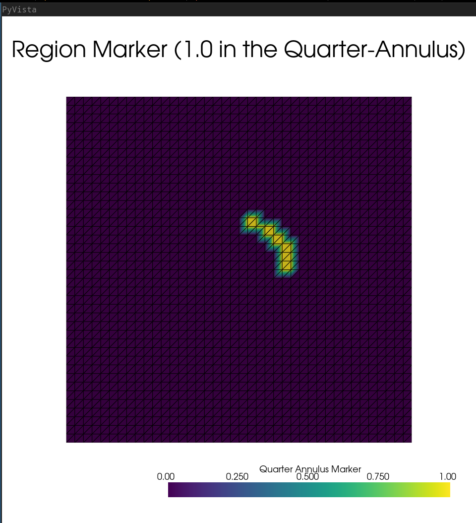
plotter.subplot(0, 1)
marker_vals = first_quadrant_marker_predicate(vis_grid_coords.T).astype(float)
grid.point_data["Region Marker"] = marker_vals
plotter.add_mesh(grid, scalars="Region Marker", show_edges=True)
plotter.add_title("Region Marker (1.0 in 1st Quad)")
plotter.view_xy()
plotter.subplot(1, 0)
s_yy_vals = marker_vals * s_yy
print(f"\n--- Sanity Check for S_yy ---")
print(f"Shape of s_yy_vals array: {s_yy_vals.shape}")
print(f"Min value: {np.min(s_yy_vals):.2e}, Max value: {np.max(s_yy_vals):.2e}")
print(f"Number of non-zero values: {np.count_nonzero(s_yy_vals)}\n")
grid.point_data["S_yy"] = s_yy_vals
plotter.add_mesh(grid, scalars="S_yy", show_edges=True, scalar_bar_args={'title': 'S_yy Value'})
plotter.add_title(f"Seebeck Tensor Component (S_yy = {s_yy:.1e})")
plotter.view_xy()
plotter.subplot(1, 1)
level_set_cg1 = fem.Function(V_cg1)
level_set_cg1.interpolate(level_set)
grid.point_data["Level Set"] = level_set_cg1.x.array
plotter.add_mesh(grid, scalars="Level Set", show_edges=True)
# CORRECTED: Use the .contour() filter method
contour = grid.contour([0.0], scalars="Level Set")
plotter.add_mesh(contour, color="red", line_width=5)
plotter.add_title("Level Set Function (<0 is inside)")
plotter.view_xy()
plotter.link_views()
plotter.show()
else:
# =============================================================================
# --- 3B. Main Solver ---
# =============================================================================
print("--- Running Main Solver ---")
dTV = ufl.TrialFunction(ME)
(u_T, u_V) = ufl.TestFunctions(ME)
TempVolt = fem.Function(ME)
(temp, volt) = ufl.split(TempVolt)
h = ufl.CellDiameter(msh)
n = ufl.FacetNormal(msh)
dx_phys = ufl.Measure("dx", subdomain_data=runtime_quadrature(level_set, "phi<0", 2 * deg), domain=msh)
gp_ids = ghost_penalty_facets(level_set, "phi<0")
gp_topo = facet_topology(msh, gp_ids)
dS_ghost = ufl.Measure("dS", subdomain_data=[(1, gp_topo)], domain=msh)
d_Gamma = ufl.Measure("dC", subdomain_data=runtime_quadrature(level_set, "phi=0", 2 * deg), domain=msh)
V_n = fem.functionspace(msh, ("DG", 1, (gdim,)))
n_level_set = fem.Function(V_n)
intersected_cells = locate_entities(level_set, tdim, "phi=0")
compute_normal(n_level_set, level_set, intersected_cells)
J_vector = -sigma * ufl.grad(volt) - sigma * Seebeck_tensor * ufl.grad(temp)
F_T = ufl.dot(kappa * ufl.grad(temp), ufl.grad(u_T)) * dx_phys
rest_terms = (ufl.dot(temp * Seebeck_tensor * J_vector, ufl.grad(u_T))
+ ufl.dot(volt * J_vector, ufl.grad(u_T))) * dx_phys
F_T += rest_terms
F_V = -ufl.dot(ufl.grad(u_V), J_vector) * dx_phys
F_ghost = (
avg(gamma_g) * avg(h) * ufl.dot(ufl.jump(ufl.grad(temp), n), ufl.jump(ufl.grad(u_T), n)) * dS_ghost(1)
+ avg(gamma_g) * avg(h) * ufl.dot(ufl.jump(ufl.grad(volt), n), ufl.jump(ufl.grad(u_V), n)) * dS_ghost(1)
)
x = ufl.SpatialCoordinate(msh)
r = ufl.sqrt(x[0]**2 + x[1]**2)
on_inner = ufl.conditional(ufl.lt(r, (R_inner + R_outer) / 2), 1, 0)
on_outer = ufl.conditional(ufl.ge(r, (R_inner + R_outer) / 2), 1, 0)
g_T = on_inner * T_cold + on_outer * T_hot
integrand_nitsche = (
-ufl.dot(kappa * ufl.grad(temp), n_level_set) * u_T
- ufl.dot(kappa * ufl.grad(u_T), n_level_set) * (temp - g_T)
+ (gamma_N * kappa / h) * (temp - g_T) * u_T
)
F_nitsche = (region_marker * integrand_nitsche) * d_Gamma
F = F_T + F_V + F_ghost + F_nitsche
J = ufl.derivative(F, TempVolt, dTV)
F_cut = cut_form(F)
J_cut = cut_form(J)
A = assemble_matrix(J_cut)
A.assemble()
b = assemble_vector(F_cut)
solver = PETSc.KSP().create(msh.comm)
solver.setOperators(A)
solver.setType(PETSc.KSP.Type.PREONLY)
solver.getPC().setType(PETSc.PC.Type.LU)
solver.getPC().setFactorSolverType("mumps")
print("--- Starting Newton Solver ---")
delta_TempVolt = fem.Function(ME)
def find_outside_dofs(subspace):
V_collapsed, dof_map = subspace.collapse()
ls_in_V = fem.Function(V_collapsed)
ls_in_V.interpolate(level_set)
local_indices_outside = np.where(ls_in_V.x.array > 0)[0]
global_dofs = np.array([dof_map[i] for i in local_indices_outside], dtype=np.int32)
return global_dofs
outside_dofs_T = find_outside_dofs(ME.sub(0))
outside_dofs_V = find_outside_dofs(ME.sub(1))
outside_dofs = np.union1d(outside_dofs_T, outside_dofs_V).astype(np.int32)
i = 0
max_it = 30
tol = 1e-8
# CORRECTED: Assemble the vector after setting values
b.setValues(outside_dofs, np.zeros_like(outside_dofs, dtype=default_scalar_type))
b.assemble()
norm_r = b.norm()
print(f"Iteration {i}: residual = {norm_r:.2e}")
while norm_r > tol and i < max_it:
A.zeroEntries()
assemble_matrix(J_cut, A=A)
A.assemble()
deactivate(A, "phi>0", level_set, [ME])
solver.setOperators(A)
assemble_vector(F_cut, b=b)
# CORRECTED: Assemble the vector after setting values
b.setValues(outside_dofs, np.zeros_like(outside_dofs, dtype=default_scalar_type))
b.assemble()
solver.solve(-b, delta_TempVolt.vector)
delta_TempVolt.x.scatter_forward()
TempVolt.x.array[:] += delta_TempVolt.x.array
TempVolt.x.scatter_forward()
i += 1
assemble_vector(F_cut, b=b)
b.setValues(outside_dofs, np.zeros_like(outside_dofs, dtype=default_scalar_type))
b.assemble()
norm_r = b.norm()
print(f"Iteration {i}: residual = {norm_r:.2e}")
if norm_r <= tol:
print(f"Converged in {i} iterations.")
else:
print("Newton solver did not converge.")
# --- Post-Processing ---
print("--- Post-Processing ---")
inside_entities = locate_entities(level_set, tdim, "phi<0")
# CORRECTED: Use the robust .collapse() method to get DoF coordinates
V_temp_collapsed, _ = ME.sub(0).collapse()
dof_coords_vis = V_temp_collapsed.tabulate_dof_coordinates()
cut_cells = cut_entities(level_set, dof_coords_vis, intersected_cells, tdim, "phi<0")
cut_mesh = create_cut_mesh(msh.comm, cut_cells, msh, inside_entities)
temp_sol = cut_function(TempVolt.sub(0), cut_mesh)
volt_sol = cut_function(TempVolt.sub(1), cut_mesh)
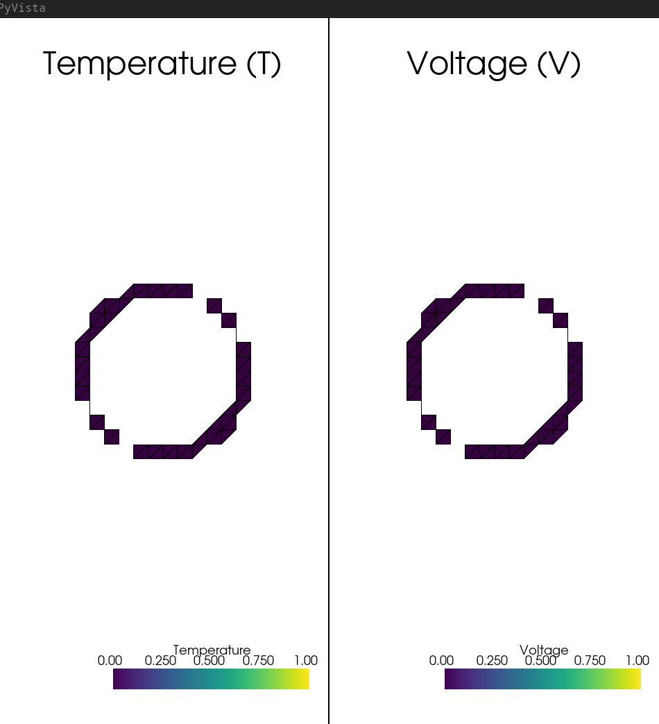
plotter = pyvista.Plotter(shape=(1, 2), window_size=[1600, 800])
plotter.subplot(0, 0)
temp_grid = pyvista.UnstructuredGrid(*plot.vtk_mesh(temp_sol.function_space))
temp_grid.point_data["Temperature"] = temp_sol.x.array
plotter.add_mesh(temp_grid, scalars="Temperature", show_edges=True)
plotter.add_title("Temperature (T)")
plotter.view_xy()
plotter.subplot(0, 1)
volt_grid = pyvista.UnstructuredGrid(*plot.vtk_mesh(volt_sol.function_space))
volt_grid.point_data["Voltage"] = volt_sol.x.array
plotter.add_mesh(volt_grid, scalars="Voltage", show_edges=True)
plotter.add_title("Voltage (V)")
plotter.view_xy()
plotter.link_views()
plotter.show()
The traceback:
--- Running Main Solver ---
Warning implementation still to be tested for mixed element
Warning implementation still to be tested for mixed element
Warning implementation still to be tested for mixed element
Warning implementation still to be tested for mixed element
Warning implementation still to be tested for mixed element
--- Starting Newton Solver ---
Iteration 0: residual = 0.00e+00
Converged in 0 iterations.
--- Post-Processing ---
Traceback (most recent call last):
  File "/home/isaac/Documents/fenicsx/Bridgman/2d_bridgman_textbook_example/debug_CutFEMx_annulus/annulus_gemini_visualizer_27_06_2025.py", line 280, in <module>
    temp_grid = pyvista.UnstructuredGrid(*plot.vtk_mesh(temp_sol.function_space))
                                          ^^^^^^^^^^^^^^^^^^^^^^^^^^^^^^^^^^^^^^
  File "/home/isaac/.conda/envs/cutfemx/lib/python3.12/functools.py", line 909, in wrapper
    return dispatch(args[0].__class__)(*args, **kw)
           ^^^^^^^^^^^^^^^^^^^^^^^^^^^^^^^^^^^^^^^^
  File "/home/isaac/.conda/envs/cutfemx/lib/python3.12/site-packages/dolfinx/plot.py", line 49, in vtk_mesh
    dim = msh.topology.dim
          ^^^^^^^^^^^^
AttributeError: 'dolfinx.cpp.fem.FunctionSpace_float64' object has no attribute 'topology'
and here’s what the visualizer produces:
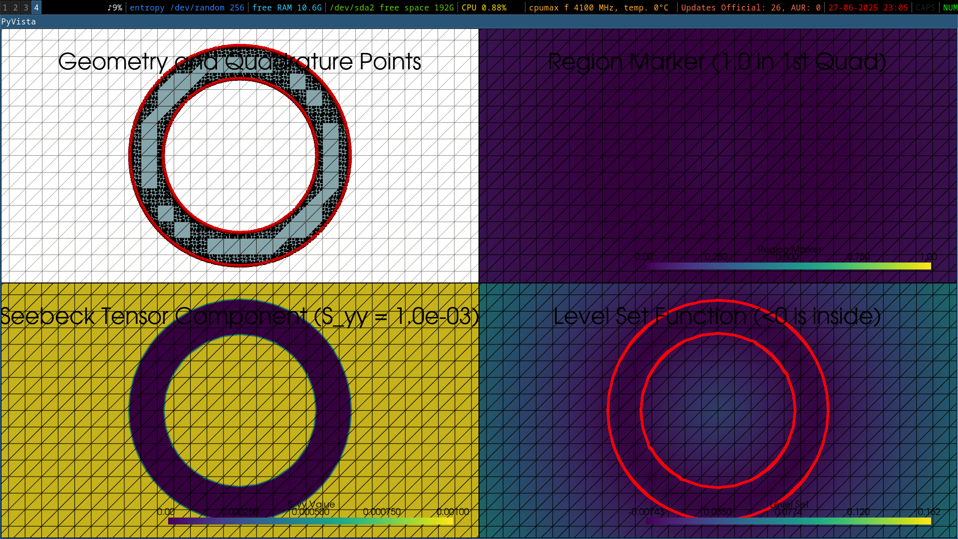
It shows all regions marked as 0 (it shouldn’t. It should mark the annulus as 1). It shows the S tensor as 0 in the whole annulus and worth 1e-3 all around it, while it should be 0 everywhere except in the 1st quadrant of the annulus region. I guess the remaining 2 figures (top left and bottom right) are correct.
Any help/guidance in debugging the code and making it work is appreciated. ![]() feel free to ask any question.
feel free to ask any question.