Hi, I have a conceptual question regarding the use of NonlinearProblem.
I’ve created a simple working example where I have a phase field driven only by a double-well.
double_well = phi**2 * (1-phi)**2
I expected all regions with initial phi > 0.5 to become phi=1, and phi<0.5 to become phi=0, except for a small boundary. However, this is not what I observe, as phi continues to decrease over time.
The image below give the initial sine condition, the observed result, and the expected result respectively:
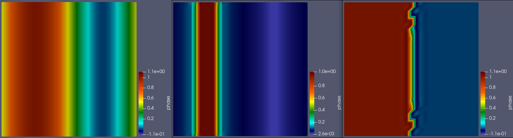
The expected result is what I obtain when I provide the derivative of the double-well, rather than the double-well term itself.
double_well_derivative = 2 * phi * (1-phi)**2 - 2 * phi**2 * (1-phi)
This is similar to how the cahn-hilliard tutorial provides the derivative of the chemical potential dfdc, rather than f itself. Why is this necessary, shouldn’t F be the function we aim to minimize, rather than its derivative?
Thank you!
Minimal example:
import numpy as np
from dolfinx import mesh, fem, io, geometry
from dolfinx.fem.petsc import NonlinearProblem
from dolfinx.nls.petsc import NewtonSolver
from dolfinx import default_real_type
from dolfinx.mesh import CellType, create_unit_square
from mpi4py import MPI
from petsc4py import PETSc
from dolfinx.io import XDMFFile
import ufl

dt = 2e-1

# Mesh
mesh_domain = create_unit_square(MPI.COMM_WORLD, 30, 30, CellType.triangle)

# Function spaces
V_a = fem.FunctionSpace(mesh_domain, ("CG", 1))
phi = fem.Function(V_a, name="phase")
phi_prev = fem.Function(V_a, name="phase_old")
v = ufl.TestFunction(V_a)

# No BCs
# Initial condition
phi.interpolate(lambda x: 0.5 + 0.5 * np.sin(x[0] * (2 * np.pi)))  # sine
phi.x.scatter_forward()

"""
Phase field formulation: F = time derivative + double well
"""
# ----- This definition does not lead to expected result: -----
# double_well = phi**2 * (1-phi)**2
# F = (phi - phi_prev) / dt * v * ufl.dx + double_well * v * ufl.dx

# ----- This does lead to expected result: -----
double_well_derivative = 2 * phi * (1-phi)**2 - 2 * phi**2 * (1-phi)
F = (phi - phi_prev) / dt * v * ufl.dx + double_well_derivative * v * ufl.dx

"""
Solver setup
"""

# Create nonlinear problem and Newton solver
problem = NonlinearProblem(F, phi)
solver = NewtonSolver(MPI.COMM_WORLD, problem)
solver.convergence_criterion = "incremental"
solver.rtol = np.sqrt(np.finfo(default_real_type).eps) * 1e-2

# We can customize the linear solver used inside the NewtonSolver by
# modifying the PETSc options
ksp = solver.krylov_solver
opts = PETSc.Options()  # type: ignore
option_prefix = ksp.getOptionsPrefix()
opts[f"{option_prefix}ksp_type"] = "preonly"
opts[f"{option_prefix}pc_type"] = "lu"
sys = PETSc.Sys()  # type: ignore
opts[f"{option_prefix}pc_factor_mat_solver_type"] = "mumps"
ksp.setFromOptions()

"""
Solving & saving
"""
file = XDMFFile(MPI.COMM_WORLD, "out.xdmf", "w")
file.write_mesh(mesh_domain)

t = 0.0
timesteps = 100

phi_prev.x.array[:] = phi.x.array
file.write_function(phi, -1)

for i in range(timesteps):
    t += dt
    r = solver.solve(phi)

    # Process & save solution
    phi_prev.x.array[:] = phi.x.array
    file.write_function(phi, i)

file.close()