Hi Community,
I’m working on a problem with periodic boundary conditions, using DOLFINx_mpc, it seems to me that the periodic boundary conditions are having some troubles to be imposed.
The original problem is a non-linear channel flow problem, so here is a MWE based on Couette flow in a straight channel, and using a Newton solver inspired by this post. With left-right periodic relation, the obtained numerical solution has flow and pressure profile on the mid-horizontal line looks like the following, while the analytical solution does not contain any pressure fluctuation. I’m concerned with the pressure fluctuations near the boundary, which seems to violate periodicity on the y-component of velocity. (which also appears in the original non-linear problem that I’m working with)
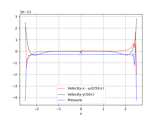
I don’t know why the periodic boundary condition is not strictly enforced with mpc.create_periodic_constraint_geometrical() in the y-component of velocity, the fluctuation is not on the scale of machine precision either. I’ve checked the periodic_boundary() and periodic_relation_left_right(), they seem to locate and map to the correct degrees of freedom. Is there something that I did wrong in specifying the boundary condition or is it something else? Any help is appreciated.
The script producing the above figure is attached below, I’m using DOLFINx 0.9.0 and DOLFINx_mpc 0.9.2.
#!/Users/tweng/miniconda3/envs/fenicsx-env/share/man/man1/python3.1
import os
import numpy as np
import tqdm.autonotebook

from mpi4py import MPI
from petsc4py import PETSc

import ufl
from basix.ufl import element, mixed_element

import dolfinx
from dolfinx import default_real_type, log
from dolfinx.mesh import create_rectangle, CellType
from dolfinx.fem import (Function, functionspace,
                         dirichletbc, locate_dofs_geometrical)
from dolfinx.io import (VTXWriter)
from dolfinx.nls.petsc import NewtonSolver
from dolfinx.fem.petsc import NonlinearProblem
import dolfinx.la as _la

import dolfinx_mpc
from dolfinx_mpc import MultiPointConstraint


############## Nonlinear MPC Problem Class ##############
# from dolfinx_mpc.problem import NonLinearProblem
class NonlinearMPCProblem(dolfinx.fem.petsc.NonlinearProblem):
    def __init__(self, F, u, mpc, bcs=[], J=None, form_compiler_options={}, jit_options={}):
        self.mpc = mpc
        super().__init__(F, u, bcs=bcs, J=J, form_compiler_options=form_compiler_options, jit_options=jit_options)

    def F(self, x: PETSc.Vec, F: PETSc.Vec):  # type: ignore
        with F.localForm() as F_local:
            F_local.set(0.0)
        dolfinx_mpc.assemble_vector(self._L, self.mpc, b=F)

        # Apply boundary condition
        dolfinx_mpc.apply_lifting(
            F,
            [self._a],
            bcs=[self.bcs],
            constraint=self.mpc,
            x0=[x],
            scale=dolfinx.default_scalar_type(-1.0),
        )
        F.ghostUpdate(addv=PETSc.InsertMode.ADD, mode=PETSc.ScatterMode.REVERSE)  # type: ignore
        dolfinx.fem.petsc.set_bc(F, self.bcs, x, -1.0)

    def J(self, x: PETSc.Vec, A: PETSc.Mat):  # type: ignore
        A.zeroEntries()
        dolfinx_mpc.assemble_matrix(self._a, self.mpc, bcs=self.bcs, A=A)
        A.assemble()


class NewtonSolverMPC(dolfinx.cpp.nls.petsc.NewtonSolver):
    def __init__(
        self,
        comm: MPI.Intracomm,
        problem: NonlinearMPCProblem,
        mpc: dolfinx_mpc.MultiPointConstraint,
    ):
        """A Newton solver for non-linear MPC problems."""
        super().__init__(comm)
        self.mpc = mpc
        self.u_mpc = dolfinx.fem.Function(mpc.function_space)

        # Create matrix and vector to be used for assembly of the non-linear
        # MPC problem
        self._A = dolfinx_mpc.cpp.mpc.create_matrix(problem.a._cpp_object, mpc._cpp_object)
        self._b = _la.create_petsc_vector(mpc.function_space.dofmap.index_map, mpc.function_space.dofmap.index_map_bs)

        self.setF(problem.F, self._b)
        self.setJ(problem.J, self._A)
        self.set_form(problem.form)
        self.set_update(self.update)

    def update(self, solver: dolfinx.nls.petsc.NewtonSolver, dx: PETSc.Vec, x: PETSc.Vec):  # type: ignore
        # We need to use a vector created on the MPC's space to update ghosts
        self.u_mpc.x.petsc_vec.array = x.array_r
        self.u_mpc.x.petsc_vec.axpy(-1.0, dx)
        self.u_mpc.x.petsc_vec.ghostUpdate(
            addv=PETSc.InsertMode.INSERT,  # type: ignore
            mode=PETSc.ScatterMode.FORWARD,  # type: ignore
        )  # type: ignore
        self.mpc.homogenize(self.u_mpc)
        self.mpc.backsubstitution(self.u_mpc)
        x.array = self.u_mpc.x.petsc_vec.array_r
        x.ghostUpdate(
            addv=PETSc.InsertMode.INSERT,  # type: ignore
            mode=PETSc.ScatterMode.FORWARD,  # type: ignore
        )  # type: ignore

    def solve(self, u: dolfinx.fem.Function):
        """Solve non-linear problem into function u. Returns the number
        of iterations and if the solver converged."""
        n, converged = super().solve(u.x.petsc_vec)
        u.x.scatter_forward()
        return n, converged

    @property
    def A(self) -> PETSc.Mat:  # type: ignore
        """Jacobian matrix"""
        return self._A

    @property
    def b(self) -> PETSc.Vec:  # type: ignore
        """Residual vector"""
        return self._b


################## System Parameters ##################
comm = MPI.COMM_WORLD
# Read from a toroidal mesh
# msh, _, facet_markers = read_from_msh(
#     "toroid.msh", MPI.COMM_WORLD, 0, gdim=2
# )
# view_mesh(msh)


Ly = 1.0
Lx = 5.0
lc = 0.05

nx = int(Lx / lc)
ny = int(Ly / lc)


# System Parameters
dt = 0.01  # time step
theta = 1  # time stepping family, e.g. theta=1 -> backward Euler, theta=0.5 -> Crank-Nicholson
omega = 1  # shear rate
num_steps = 10

output_dir = "testCouette_mix_Ly1Lx1r0.1_omega1_dt1e-2_t0.1"

# Save all logging to file
log.set_output_file(
    os.path.join(output_dir, "log.txt")
)


################# Mesh Creation #################
msh = create_rectangle(comm=comm,
                       points=[[-Lx/2, -Ly/2], [Lx/2, Ly/2]],
                       n=[nx, ny],
                       cell_type=CellType.triangle,
                       dtype=default_real_type)

# Create the Taylot-Hood function space
P2 = element("Lagrange", msh.basix_cell(), 2, shape=(msh.geometry.dim,), dtype=default_real_type)
P1 = element("Lagrange", msh.basix_cell(), 1, dtype=default_real_type)

# Create the mixed element space for the Q-equation
TH = mixed_element([P2, P1])
W = functionspace(msh, TH)


################# Boundary Conditions ###########

# No slip boundary condition on the collapsed Taylot-Hood function space
W0 = W.sub(0)
V, _ = W0.collapse()

fdim = msh.topology.dim - 1
wall_marker = 3
# Outer boundary: no-slip condition

def noslip_boundary(x):
    return np.isclose(x[1], Ly/2)

def shear_boundary(x):
    return np.isclose(x[1], -Ly/2)

u_noslip = Function(V)
u_noslip.x.array[:] = 0.0
bcu_walls = dirichletbc(
    u_noslip,
    locate_dofs_geometrical(
        (W0, V),
        noslip_boundary
        ),
    W0)

def shear_expression(x):
    return np.stack((omega * np.ones(x.shape[1]), np.zeros(x.shape[1])))

u_shear = Function(V)
u_shear.interpolate(shear_expression)
bcu_shear = dirichletbc(
    u_shear,
    locate_dofs_geometrical(
        (W0, V),
        shear_boundary
        ),
    W0)


P, _ = W.sub(1).collapse()
point = Function(P)
point.x.array[:] = 0.0
p_point = dirichletbc(
    point,
    locate_dofs_geometrical(
        (W.sub(1), P),
        lambda x: np.isclose(x.T, [0, 0, 0]).all(axis=1)
    ),
    W.sub(1)
)

# Collect Dirichlet boundary conditions
bcs = [bcu_walls, bcu_shear, p_point]
# bcs = [bcu_walls, bcu_shear]

def periodic_boundary(x):
    tol = 1000 * np.finfo(x.dtype).resolution
    return np.isclose(x[0], Lx/2, atol=tol) & (x[1] != -Ly/2) & (x[1] != Ly/2)

def periodic_relation_left_right(x):
    out_x = np.zeros(x.shape)
    out_x[0] = x[0] - Lx
    out_x[1] = x[1]
    out_x[2] = x[2]
    return out_x

mpc = MultiPointConstraint(W)
for i in range(W.num_sub_spaces):
    # Create a MultiPointConstraint for the periodic boundary condition
    mpc.create_periodic_constraint_geometrical(
        W.sub(i),
        periodic_boundary,
        periodic_relation_left_right,
        bcs,
        scale=1.0,
    )
mpc.finalize()


W_mpc = mpc.function_space


################## Initial Conditions ##################

w = Function(W_mpc) # Function representing the solution
w0 = Function(W_mpc) # Function representing the solution of the previous step

# Interpolate initial conditions
w.x.array[:] = 0.0
# rng = np.random.default_rng(seed=42)
# w.sub(2).interpolate(lambda x: [0.002 * (rng.random(x.shape[1])), 0.002 * (rng.random(x.shape[1]))])
w.x.scatter_forward()
# mpc.homogenize(w)

##################### Weak Formulation #####################

# Splitting the functions for setting up the variational forms
(u, p) = ufl.split(w)
(u0, p0) = ufl.split(w0)

(ut, pt)= ufl.TestFunctions(W)

F2 = (
    ufl.inner(ufl.grad(u), ufl.grad(ut)) * ufl.dx - p * ufl.div(ut) * ufl.dx
)

F3 = (ufl.dot(u, ufl.grad(pt)) * ufl.dx)

F = F2 + F3

J = ufl.derivative(F, w, ufl.TrialFunction(W))

# setup Q solver
solver2 = NewtonSolverMPC(MPI.COMM_WORLD, NonlinearMPCProblem(F, w, mpc=mpc, bcs=bcs, J=J), mpc=mpc)
solver2.convergence_criterion = "incremental"
solver2.rtol = 1e-10
solver2.atol = 1e-9
solver2.relaxation_parameter = 1
solver2.max_it = 100


ksp2 = solver2.krylov_solver
opts2 = PETSc.Options()  # type: ignore
option_prefix = ksp2.getOptionsPrefix()
opts2[f"{option_prefix}ksp_type"] = "cg"
opts2[f"{option_prefix}ksp_rtol"] = "5.3e-12"
opts2[f"{option_prefix}pc_type"] = "lu"
opts2[f"{option_prefix}pc_factor_mat_solver_type"] = "mumps"
# opts2[f"{option_prefix}pc_type"] = "hypre"
# opts2[f"{option_prefix}pc_hypre_type"] = "boomeramg"
# opts2[f"{option_prefix}pc_hypre_boomeramg_max_iter"] = 1
# opts2[f"{option_prefix}pc_hypre_boomeramg_cycle_type"] = "v"
ksp2.setFromOptions()

# Setup output format before time integration
t = 0.0

V1, _ = W_mpc.sub(0).collapse()
u_ = Function(V1)
u_.interpolate(w.sub(0).collapse())
u_.name = "Velocity"

Q1, _ = W_mpc.sub(1).collapse()
p_ = Function(Q1)
p_.interpolate(w.sub(1).collapse())
p_.name = "Pressure"

from pathlib import Path
folder = Path(output_dir)
folder.mkdir(exist_ok=True, parents=True)

vtx_u = VTXWriter(msh.comm, os.path.join(folder, "u.bp"), [u_], engine="BP4")
vtx_p = VTXWriter(msh.comm, os.path.join(folder, "Q.bp"), [p_], engine="BP4")

vtx_u.write(t)
vtx_p.write(t)

progress = tqdm.autonotebook.tqdm(desc="Solving PDE", total=num_steps)
for i in range(num_steps):
    progress.update(1)
    # Update current time step
    t += dt
    log.set_log_level(log.LogLevel.DEBUG)

    # Step 2: Q solver
    n, converged = solver2.solve(w)
    assert (converged)
    w.x.scatter_forward()
    w0.x.array[:] = w.x.array

    (u, p) = ufl.split(w)

    u_.interpolate(w.sub(0).collapse())
    p_.interpolate(w.sub(1).collapse())

    # Write solutions to file
    vtx_u.write(t)
    vtx_p.write(t)

progress.close()
vtx_u.close()
vtx_p.close()

############## Plot the Horizontal Profile ##############
tol = 0.001  # Avoid hitting the outside of the domain
x = np.linspace(-Lx/2 + tol, Lx/2 - tol, 101)
points = np.zeros((3, 101))
points[0] = x
u_values = []
p_values = []

bb_tree = dolfinx.geometry.bb_tree(msh, msh.topology.dim)
cells = []
points_on_proc = []
# Find cells whose bounding-box collide with the the points
cell_candidates = dolfinx.geometry.compute_collisions_points(bb_tree, points.T)
# Choose one of the cells that contains the point
colliding_cells = dolfinx.geometry.compute_colliding_cells(msh, cell_candidates, points.T)
for i, point in enumerate(points.T):
    if len(colliding_cells.links(i)) > 0:
        points_on_proc.append(point)
        cells.append(colliding_cells.links(i)[0])

points_on_proc = np.array(points_on_proc, dtype=np.float64)
ux_values = u_.eval(points_on_proc, cells)[:,0] - omega / 2
uy_values = u_.eval(points_on_proc, cells)[:,1]
p_values = p_.eval(points_on_proc, cells)

import matplotlib.pyplot as plt
fig = plt.figure()
plt.plot(points_on_proc[:, 0], ux_values, "k-.", linewidth=1, label="Velocity-x - $\omega/2$")
plt.plot(points_on_proc[:, 0], uy_values, "k--", linewidth=1, label="Velocity-y")
plt.plot(points_on_proc[:, 0], p_values, "b--", linewidth=1, label="Pressure")
plt.grid(True)
plt.xlabel("x")
plt.legend()
# If run in parallel as a python file, we save a plot per processor
plt.savefig(f"periodicity_rank{MPI.COMM_WORLD.rank:d}.png")