Hi Dolfinx community!
I noticed an interesting behaviour while working with mixed-element function spaces for
multiphysics problems. In most examples (As in this community post or Dokken’s example here), we see mixed element function spaces where the elements are different:
    PE = basix.ufl.element('CG', mesh.basix_cell(), degree=1)
    QE = basix.ufl.element('CG', mesh.basix_cell(), degree=1, shape=(mesh.topology.dim,))
    ME = basix.ufl.mixed_element([QE, PE])
    W = dolfinx.fem.functionspace(mesh, ME)
When applying boundary conditions, we need to find the DOFs associated with the collapsed space:
    u_sub, u_submap = W.sub(0).collapse()
    p_sub, p_submap = W.sub(1).collapse()
    dofs_L = dolfinx.fem.locate_dofs_topological((W.sub(0), U_sub), fdim, boundary.find(1))
I have noticed odd behaviour when working with mixed-element function spaces where the elements are
of the same type:
    PE = basix.ufl.element('CG', mesh.basix_cell(), degree=1)
    ME = basix.ufl.mixed_element([PE, PE])
    W = dolfinx.fem.functionspace(mesh, ME)
Specifically, I have seen the following:
- I don’t need to collapse the sub space (W.sub(0)) when finding the dofs.
- If I do collapse the sub space, I notice the solution field has zeros near the boundary that I apply the condition to (see below).
COLLAPSED:
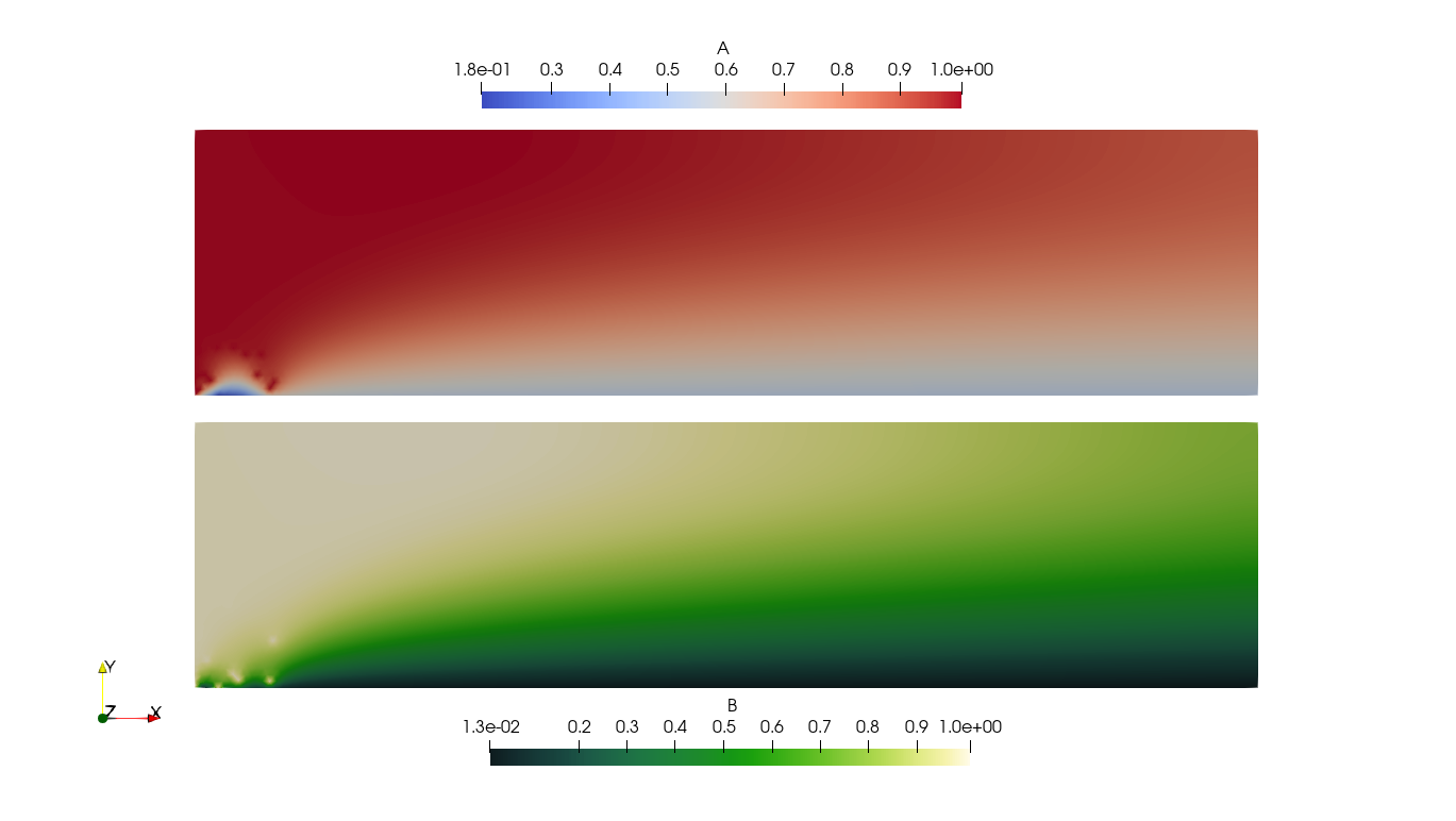
NON COLLAPSED
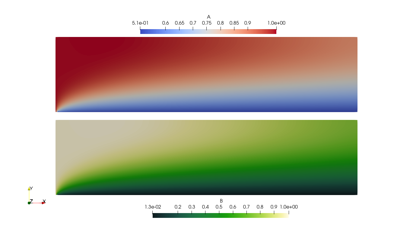
In many circumstances, I can solve the problems by collapsing when there are different elements in the mixed function space ([QE, PE]) and not collapsing when the sub-elements are the same ([PE, PE]); however, I would like to be able to generalize the approach for mixed physics (i.e. fluid flow with 2 species reactions, solved monolithically).
If I’m understanding correctly, collapsing the subspace is the correct way of applying dofs. Any help identifying why errors are introduced when collapsing subspaces of the same element or how to work around that is much appreciated!!
Here is a coupled two species ADR code that I am testing on. This example is a simplification (2-species, no stabilization) from a demo my team created for a Dolfin 2019 wrapper (here). This code produced the images shown above. I understand this is long for a MWE - but I’m trying to show the context and both approaches.
from dolfinx.fem import petsc
from dolfinx.io import gmshio
from dolfinx.nls.petsc import NewtonSolver
from mpi4py import MPI

import basix
import dolfinx
import numpy as np
import ufl

def advective_form(c, u, w, domain):
    return w * ufl.inner(u, ufl.grad(c)) * domain

def diffusive_form(c, D, w, domain):
    return D * ufl.inner(ufl.grad(w), ufl.grad(c)) * domain

def reactive_form(r, w, domain):
    return w * r * domain

def write_solution(sol, output_dir='output'):
    c_A = sol.split()[0].collapse()
    c_B = sol.split()[1].collapse()
    c_A.name = 'A'
    c_B.name = 'B'
    A_file = dolfinx.io.VTKFile(MPI.COMM_WORLD, f'{output_dir}/solution_A.pvd', 'w')
    B_file = dolfinx.io.VTKFile(MPI.COMM_WORLD, f'{output_dir}/solution_B.pvd', 'w')
    A_file.write_function(c_A)
    B_file.write_function(c_B)

def main():
    # Define mesh
    mesh, subdomain, boundary = gmshio.read_from_msh('rect.msh', comm=MPI.COMM_WORLD, gdim=2)
    # Problem specific constants
    n = ufl.FacetNormal(mesh)
    D = dolfinx.fem.Constant(mesh, dolfinx.default_scalar_type(0.1))
    k_v = dolfinx.fem.Constant(mesh, dolfinx.default_scalar_type(0.01))
    k_s = dolfinx.fem.Constant(mesh, dolfinx.default_scalar_type(1.0))
    c0 = dolfinx.fem.Constant(mesh, dolfinx.default_scalar_type(1.0))
    zero = dolfinx.fem.Constant(mesh, dolfinx.default_scalar_type(0.0))
    u_mag = 10.0

    # Domain measures
    x = ufl.SpatialCoordinate(mesh)
    dx = ufl.Measure('dx', metadata={'quadrature_degree': 5}, domain=mesh)
    ds = ufl.Measure('ds', domain=mesh, subdomain_data=boundary, metadata={'quadrature_degree': 5})
    u = ufl.as_vector([u_mag * x[1] * (1 - x[1]), 0.0])

    # Define function space, test and solution functions
    poly_element = basix.ufl.element('CG', mesh.basix_cell(), 1)
    mixed_element = basix.ufl.mixed_element([poly_element, poly_element])
    V = dolfinx.fem.functionspace(mesh, mixed_element)
    ```
    sol = dolfinx.fem.Function(V)
    sol_A, sol_B = ufl.split(sol)

    w = ufl.TestFunction(V)
    w_A, w_B = ufl.split(w)

    # Define the weak form
    A_form = (advective_form(sol_A, u, w_A, dx) + diffusive_form(sol_A, D, w_A, dx) + reactive_form(-k_v * sol_A * sol_B, w_A, dx))
    flux_A = -k_s * sol_A * sol_B / D * n
    A_form += -w_A * ufl.dot(flux_A, n) * ds(2)
    B_form = (advective_form(sol_B, u, w_B, dx) + diffusive_form(sol_B, D, w_B, dx) + reactive_form(-2 * k_v * sol_A * sol_B, w_B, dx))
    flux_B = -2 * k_s * sol_A * sol_B / D * n
    B_form += -w_B * ufl.dot(flux_B, n) * ds(2)

    monolithic_form = A_form + B_form

    # IMPLEMENTATION ONE - COLLAPSED FUNCTION SPACES (errors)
    V_A = V.sub(0)
    V_B = V.sub(1)
    V_A_sub, V_A_submap = V_A.collapse()
    V_B_sub, V_B_submap = V_B.collapse()
    V_dof_search_A = (V_A, V_A_sub)
    V_dof_search_B = (V_B, V_B_sub)

    dofs_A = np.concatenate(dolfinx.fem.locate_dofs_topological(V_dof_search_A, entity_dim=1, entities=boundary.find(1)))
    dofs_B = np.concatenate(dolfinx.fem.locate_dofs_topological(V_dof_search_B, entity_dim=1, entities=boundary.find(1)))

    bc_A = dolfinx.fem.dirichletbc(c0, dofs_A, V_A)
    bc_B = dolfinx.fem.dirichletbc(c0, dofs_B, V_B)
    bcs = [bc_A, bc_B]

    # Set up problem
    c = ufl.TrialFunction(V)
    problem = petsc.NonlinearProblem(F=monolithic_form, u=sol, bcs=bcs, J=ufl.derivative(monolithic_form, sol, c))
    solver = NewtonSolver(MPI.COMM_WORLD, problem)

    num_iterations, converged = solver.solve(sol)
    write_solution(sol, 'output-collapsed')

    # IMPLEMENTATION TWO - NON-COLLAPSED FUNCTION SPACES (smooth)
    V_A = V.sub(0)
    V_B = V.sub(1)
    dofs_A = dolfinx.fem.locate_dofs_topological(V_A, entity_dim=1, entities=boundary.find(1))
    dofs_B = dolfinx.fem.locate_dofs_topological(V_B, entity_dim=1, entities=boundary.find(1))
    bc_A = dolfinx.fem.dirichletbc(c0, dofs_A, V_A)
    bc_B = dolfinx.fem.dirichletbc(c0, dofs_B, V_B)
    bcs = [bc_A, bc_B]

    c = ufl.TrialFunction(V)
    problem = petsc.NonlinearProblem(F=monolithic_form, u=sol, bcs=bcs, J=ufl.derivative(monolithic_form, sol, c))
    solver = NewtonSolver(MPI.COMM_WORLD, problem)

    num_iterations, converged = solver.solve(sol)
    write_solution(sol, 'output-non-collapsed')

if __name__ == "__main__":
    main()
Here is the gmsh script to generate the mesh. Also note that this problem persist regardless of the mesh generation technique (dolfinx, gmsh, or xdmf).
    h = 0.03;
    Point(1) = {0, 0, 0, h};
    Point(2) = {4, 0, 0, h};
    Point(3) = {4, 1, 0, h};
    Point(4) = {0, 1, 0, h};
    Line(1) = {4, 3};
    Line(2) = {3, 2};
    Line(3) = {2, 1};
    Line(4) = {1, 4};
    Curve Loop(1) = {1, 2, 3, 4};
    Plane Surface(1) = {1};
    Physical Curve(1) = {4};
    Physical Curve(4) = {1};
    Physical Curve(3) = {2};
    Physical Curve(2) = {3};
    Physical Surface(1) = {1};