Difference of DirichletBC of Nedelec elements between dolfin and dolfinx

Hello. I am a new user of dolfinx and I am trying to convert the code in this link, from dolfin to dolfinx. The code in dolfinx is:


from mpi4py import MPI
from dolfinx import mesh, fem, plot
from dolfinx.fem import FunctionSpace, Function, Constant, Expression, dirichletbc, VectorFunctionSpace
import numpy as np
from petsc4py import PETSc
from petsc4py.PETSc import ScalarType
import ufl
from ufl import TrialFunction, TestFunction
import pyvista
import dolfinx
import gmsh
from dolfinx.io import gmshio

gmsh.initialize()
Sphere = gmsh.model.occ.addSphere(0, 0, 0, 1, 1)
gmsh.model.occ.synchronize()
Geometry_Dimension = 3
volumes = gmsh.model.getEntities(Geometry_Dimension)
Volume_Physical_Tag = 1
Volume_Physical = gmsh.model.addPhysicalGroup(volumes[0][0], [volumes[0][1]], Volume_Physical_Tag)
gmsh.model.mesh.field.add("Ball", 1)
gmsh.model.mesh.field.setNumber(1, "VIn", 0.1)
gmsh.model.mesh.field.setNumber(1, "XCenter", 0)
gmsh.model.mesh.field.setNumber(1, "YCenter", 0)
gmsh.model.mesh.field.setNumber(1, "ZCenter", 0)
gmsh.model.mesh.field.setNumber(1, "Radius", 1)
gmsh.model.mesh.field.add("Min", 2)
gmsh.model.mesh.field.setNumbers(2, "FieldsList", [1])
gmsh.model.mesh.field.setAsBackgroundMesh(2)
gmsh.model.mesh.generate(3)
mesh_comm = MPI.COMM_WORLD
model_rank = 0
domain, cell_tags, facet_tags = gmshio.model_to_mesh(gmsh.model, mesh_comm, model_rank, Geometry_Dimension)

# Define function spaces
V = FunctionSpace(domain, ("Nedelec 1st kind H(curl)", 1))

# Define test and trial functions
v = TestFunction(V)
u = TrialFunction(V)

# Define functions for boundary condiitons
dbdt = Constant(domain, (0.0, 0.0, 1.0))

zero = fem.Function(V)
zero_val = fem.Constant(domain, PETSc.ScalarType([0.0, 0.0, 0.0]))
zero_expr = fem.Expression(zero_val, V.element.interpolation_points())
zero.interpolate(zero_expr)

# Magnetic field (to be computed)
T = Function(V)

# Dirichlet boundary condition
tdim = domain.topology.dim
fdim = tdim - 1
domain.topology.create_connectivity(fdim, tdim)
boundary_facets = mesh.exterior_facet_indices(domain.topology)
boundary_dofs = fem.locate_dofs_topological(V, fdim, boundary_facets)
bc = dirichletbc(zero, boundary_dofs)

# Forms for the eddy-current equation
a = ufl.inner(ufl.curl(v), ufl.curl(u))*ufl.dx
L = -ufl.inner(v, dbdt)*ufl.dx

a_assembled = fem.petsc.assemble_matrix(fem.form(a), bcs = [bc])
a_assembled.assemble()

L_assembled = fem.petsc.assemble_vector(fem.form(L))
L_assembled.assemble()

# Create PETSc Krylov solver (from petsc4py)
ksp = PETSc.KSP()
ksp.create(PETSc.COMM_WORLD)

# Set the Krylov solver type and set tolerances
ksp.setType("cg")
ksp.setTolerances(rtol=1.0e-08, atol=1.0e-12, divtol=1.0e10, max_it=300)

# Get the preconditioner and set type (HYPRE AMS)
pc = ksp.getPC()
pc.setType("hypre")
pc.setHYPREType("ams")

# Build discrete gradient
P1 = FunctionSpace(domain, ("CG", 1))
G = dolfinx.cpp.fem.petsc.discrete_gradient(P1._cpp_object, V._cpp_object)
G.assemble()

# Attach discrete gradient to preconditioner
pc.setHYPREDiscreteGradient(G)

# Build constants basis for the Nedelec space
constants = [fem.Function(V) for i in range(3)]
for i, c in enumerate(constants):
    direction = Constant(domain, [1.0 if i == j else 0.0 for j in range(3)])
    c_expr = Expression(direction , V.element.interpolation_points())
    c.interpolate(c_expr)

# Inform preconditioner of constants in the Nedelec space
cvecs = [constant.vector for constant in constants]
pc.setHYPRESetEdgeConstantVectors(cvecs[0], cvecs[1], cvecs[2])

# We are dealing with a zero conductivity problem (no mass term), so
# we need to tell the preconditioner
pc.setHYPRESetBetaPoissonMatrix(None)

# Set operator for the linear solver
ksp.setOperators(a_assembled)

# Set options prefix
ksp.setOptionsPrefix("eddy_")

# Turn on monitoring of residual
opts = PETSc.Options()
opts.setValue("-eddy_ksp_monitor_true_residual", None)

# Solve eddy currents equation (using potential T)
ksp.setFromOptions()
ksp.solve(L_assembled, T.vector)

# Test and trial functions for density equation
W = VectorFunctionSpace(domain, ("CG", 1))
v2 = TestFunction(W)
u2 = TrialFunction(W)

# Solve density equation (use conjugate gradient linear solver)
J = Function(W)
a2 = ufl.inner(v2, u2)*ufl.dx
L2 = ufl.inner(v2, ufl.curl(T))*ufl.dx
problem = fem.petsc.LinearProblem(a2, L2, petsc_options={"linear_solver": "cg"})
J = problem.solve()

However, by plotting J, the result on the boundary nodes are not match with the result from dolfin. The current density resulted from dolfin is shown in the image below.

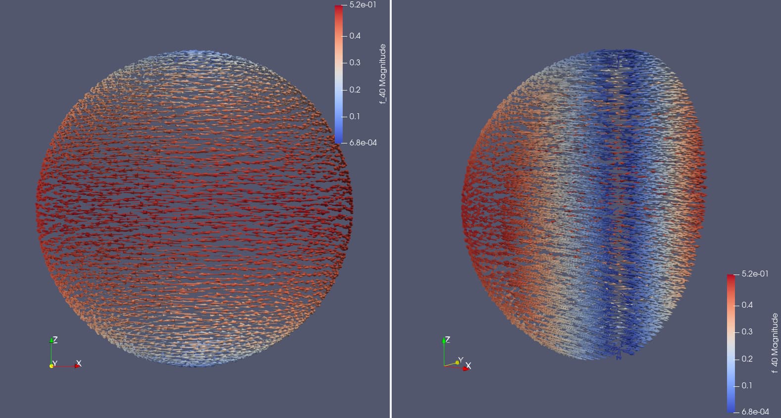
The result from dolfinx is also shown in the image below.

Although the current density calculated for inner elements seems to be identical, but the result on the boundary is not correct in the code of dolfinx. I am wondering what the problem is and how I can fix my code. I would be so grateful if you could please help me in this regard.
Thank you in advance for your guidance.

I would suggest you have a look at: https://github.com/jpdean/maxwell/blob/master/solver.py
The Nedelec elements in DOLFINx is properly implemented wrt interpolation, meaning that the functionals described the basis functions are integral moments, not point evaluations, as in the case of legacy dolfin. The effect of this is optimal interpolation properties.

You can Also see: Magnetostatics 3D - wrong 3D magnetic vector potential - #5 by ftrillaudp

1 Like

Dear Dokken,
Thanks for the response. It helped and now I can solve the reference problem from dolfin in dolfinx. However, when I tried to use this method for my problem, which the right hand side of the weak formulation is not constant, the solver cannot converge. For example, in the minimal example below, when dbdt is constant (line 57), the code works properly, but when it is defined as a function varying with respect to spatial coordinate (line 58 and 59), the problem cannot be solved.

import dolfinx
import gmsh
import ufl
import pyvista
import numpy as np
from mpi4py import MPI
from dolfinx import mesh, fem, plot
from dolfinx.io import gmshio
from dolfinx.fem import FunctionSpace, Function, Constant, Expression, dirichletbc, VectorFunctionSpace, form, locate_dofs_topological, petsc
from dolfinx.mesh import Mesh
from dolfinx.common import Timer, timing
from dolfinx.cpp.fem.petsc import discrete_gradient, interpolation_matrix
from ufl import TrialFunction, TestFunction, VectorElement, curl, dx, inner
from ufl.core.expr import Expr
from petsc4py import PETSc
from petsc4py.PETSc import ScalarType
from typing import Dict


try:
    gmsh.initialize()
    gmsh.clear()
except:
    gmsh.clear()
Sphere = gmsh.model.occ.addSphere(0, 0, 0, 1, 1)
gmsh.model.occ.synchronize()
Geometry_Dimension = 3
volumes = gmsh.model.getEntities(Geometry_Dimension)
Volume_Physical_Tag = 1
Volume_Physical = gmsh.model.addPhysicalGroup(volumes[0][0], [volumes[0][1]], Volume_Physical_Tag)
boundary_marker = 2
boundary = gmsh.model.getBoundary(volumes, oriented=False)
gmsh.model.addPhysicalGroup(boundary[0][0], [boundary[0][1]], boundary_marker, "boundary physical")
gmsh.model.mesh.field.add("Ball", 1)
gmsh.model.mesh.field.setNumber(1, "VIn", 0.05)
gmsh.model.mesh.field.setNumber(1, "XCenter", 0)
gmsh.model.mesh.field.setNumber(1, "YCenter", 0)
gmsh.model.mesh.field.setNumber(1, "ZCenter", 0)
gmsh.model.mesh.field.setNumber(1, "Radius", 1)
gmsh.model.mesh.field.add("Min", 2)
gmsh.model.mesh.field.setNumbers(2, "FieldsList", [1])
gmsh.model.mesh.field.setAsBackgroundMesh(2)
gmsh.model.mesh.generate(3)
mesh_comm = MPI.COMM_WORLD
model_rank = 0
domain, cell_tags, facet_tags = gmshio.model_to_mesh(gmsh.model, mesh_comm, model_rank, Geometry_Dimension)

# Define function spaces
V = FunctionSpace(domain, ("Nedelec 1st kind H(curl)", 1))
W = VectorFunctionSpace(domain, ("CG", 1))

# Define test and trial functions
v = TestFunction(V)
u = TrialFunction(V)

# Define functions for boundary condiitons
# dbdt = Constant(domain, (0.0, 0.0, 1.0))
dbdt = Function(W)
dbdt.interpolate(lambda x: [x[0] * np.ones(x.shape[1]), np.ones(x.shape[1]), np.zeros(x.shape[1])])

zero = fem.Function(V)
zero_val = fem.Constant(domain, PETSc.ScalarType([0.0, 0.0, 0.0]))
zero_expr = fem.Expression(zero_val, V.element.interpolation_points())
zero.interpolate(zero_expr)

def solve_problem(domain: Mesh, k: int, alpha: np.float64, beta: np.float64,
                  f: Expr, boundary_marker, u_bc_ufl,
                  preconditioner: str = "ams", jit_options: Dict = None,
                  form_compiler_options: Dict = None, petsc_options: Dict = None):
    
    if form_compiler_options is None:
        form_compiler_options = {}
    if jit_options is None:
        jit_options = {}
    if petsc_options is None:
        petsc_options = {}

    V = FunctionSpace(domain, ("N1curl", k))
    ndofs = V.dofmap.index_map.size_global * V.dofmap.index_map_bs

    u = TrialFunction(V)
    v = TestFunction(V)

    alpha = Constant(domain, alpha)
    beta = Constant(domain, beta)
    a = form(inner(alpha * curl(u), curl(v)) * dx + inner(beta * u, v) * dx,
             form_compiler_options=form_compiler_options, jit_options=jit_options)

    L = form(inner(f, v) * dx,
             form_compiler_options=form_compiler_options, jit_options=jit_options)

    u = Function(V)

    tdim = domain.topology.dim
    fdim = tdim - 1
    domain.topology.create_connectivity(fdim, tdim)
    boundary_facets = mesh.exterior_facet_indices(domain.topology)
    boundary_dofs = locate_dofs_topological(
        V, entity_dim=tdim - 1, entities=boundary_facets)
    u_bc_expr = Expression(u_bc_ufl, V.element.interpolation_points())
    with Timer(f"~{k}, {ndofs}: BC interpolation"):
        u_bc = Function(V)
        u_bc.interpolate(u_bc_expr)
    bc = dirichletbc(u_bc, boundary_dofs)

    # TODO More steps needed here for Dirichlet boundaries
    with Timer(f"~{k}, {ndofs}: Assemble LHS and RHS"):
        A = petsc.assemble_matrix(a, bcs=[bc])
        A.assemble()
        b = petsc.assemble_vector(L)
        petsc.apply_lifting(b, [a], bcs=[[bc]])
        b.ghostUpdate(addv=PETSc.InsertMode.ADD,
                      mode=PETSc.ScatterMode.REVERSE)
        petsc.set_bc(b, [bc])

    # Create solver
    ksp = PETSc.KSP().create(domain.comm)
    ksp.setOptionsPrefix(f"ksp_{id(ksp)}")
    # ksp.setNormType(ksp.NormType.NORM_PRECONDITIONED)

    pc = ksp.getPC()
    opts = PETSc.Options()
    option_prefix = ksp.getOptionsPrefix()
    opts.prefixPush(option_prefix)
    for option, value in petsc_options.items():
        opts[option] = value
    opts.prefixPop()
    if preconditioner == "ams":
        pc.setType("hypre")
        pc.setHYPREType("ams")

        # Build discrete gradient
        with Timer(f"~{k}, {ndofs}: Build discrete gradient"):
            V_CG = FunctionSpace(domain, ("CG", k))._cpp_object
            G = discrete_gradient(V_CG, V._cpp_object)
            G.assemble()
            pc.setHYPREDiscreteGradient(G)

        if k == 1:
            with Timer(f"~{k}, {ndofs}: Build EdgeConstantVectors"):
                cvec_0 = Function(V)
                cvec_0.interpolate(lambda x: np.vstack((np.ones_like(x[0]),
                                                        np.zeros_like(x[0]),
                                                        np.zeros_like(x[0]))))
                cvec_1 = Function(V)
                cvec_1.interpolate(lambda x: np.vstack((np.zeros_like(x[0]),
                                                        np.ones_like(x[0]),
                                                        np.zeros_like(x[0]))))
                cvec_2 = Function(V)
                cvec_2.interpolate(lambda x: np.vstack((np.zeros_like(x[0]),
                                                        np.zeros_like(x[0]),
                                                        np.ones_like(x[0]))))
                pc.setHYPRESetEdgeConstantVectors(cvec_0.vector,
                                                  cvec_1.vector,
                                                  cvec_2.vector)
        else:
            # Create interpolation operator
            with Timer(f"~{k}, {ndofs}: Build interpolation matrix"):
                Vec_CG = FunctionSpace(domain, VectorElement("CG", domain.ufl_cell(), k))
                Pi = interpolation_matrix(Vec_CG._cpp_object, V._cpp_object)
                Pi.assemble()

                # Attach discrete gradient to preconditioner
                pc.setHYPRESetInterpolations(domain.geometry.dim, None, None, Pi, None)

        # If we are dealing with a zero conductivity problem (no mass
        # term),need to tell the preconditioner
        if np.isclose(beta.value, 0):
            pc.setHYPRESetBetaPoissonMatrix(None)

    elif preconditioner == "gamg":
        pc.setType("gamg")

    # Set matrix operator
    ksp.setOperators(A)

    def monitor(ksp, its, rnorm):
        if domain.comm.rank == 0:
            print("Iteration: {}, rel. residual: {}".format(its, rnorm))
    ksp.setMonitor(monitor)
    ksp.setFromOptions()
    pc.setUp()
    ksp.setUp()

    # Compute solution
    with Timer(f"~{k}, {ndofs}: Solve Problem"):
        ksp.solve(b, u.vector)
        u.x.scatter_forward()

    reason = ksp.getConvergedReason()
    print(f"Convergence reason {reason}")
    if reason < 0:
        u.name = "A"
        raise RuntimeError("Solver did not converge.")
    # ksp.view()
    return (u, {"ndofs": ndofs,
                "solve_time": timing(f"~{k}, {ndofs}: Solve Problem")[1],
                "iterations": ksp.its})


T, solver_data = solve_problem(domain=domain, k = 1, alpha = 1.0, beta = 0.0, f = dbdt, boundary_marker = boundary_marker, u_bc_ufl = zero)

# Test and trial functions for density equation
v2 = TestFunction(W)
u2 = TrialFunction(W)

# Solve density equation (use conjugate gradient linear solver)
J = Function(W)
a2 = ufl.inner(v2, u2)*ufl.dx
L2 = ufl.inner(v2, ufl.curl(T))*ufl.dx
problem = fem.petsc.LinearProblem(a2, L2, petsc_options={"linear_solver": "cg"})
J = problem.solve()

# Plot J
pyvista.start_xvfb()
topology, cell_types, geometry = plot.create_vtk_mesh(W)
grid = pyvista.UnstructuredGrid(topology, cell_types, geometry)
Plotter = pyvista.Plotter(window_size=[1000, 500])
Plotter_Actor1 = Plotter.add_mesh(grid, style="wireframe", line_width=2, color="k")
grid.point_data["J"] = J.vector.array.reshape(geometry.shape[0], W.dofmap.index_map_bs)
Plotter_glyphs = grid.glyph(orient="J", factor=0.2)
Plotter_Actor1 = Plotter.add_mesh(Plotter_glyphs)
Plotter.view_xz()
Plotter.show()

How can I solve a problem which the right hand side of the equation is not constant?
I am so grateful for your kind answers.

Hello. Regarding my previous post, I need to mention that I understood that the right hand side of the equation must be divergence-free and by fixing that, the problem was solved. Thanks for your help again.