Hello,
I’m working with a linear elastic structure and after solving the equilibrium problem, I need to calculate it’s strain energy. I’m also projecting the energy on DG0 space to see its distribution. However, I’m getting very different results when working with different mesh refinements and I cannot understand why.
The mesh i’m working with is always rectangular and the domain of interest is a subset of this domain. This domains are identified with a level set strategy and the complementary part of the domain is associated with very small material proprieties.
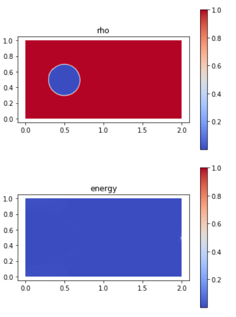
For exemple, this is what I get with a 60 x 30 mesh:
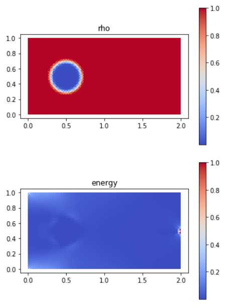
and this with a 240 x 120 mesh:
If the domain is still 2 x 1, why is it so different and concentrated on the more refined mesh? Could it be an implementation problem or is it expected? If anyone could help me, I would be really gratefull.
Here is a minimal working example:
from dolfin import *
import numpy as np
from matplotlib import pyplot as plt
from tabulate import tabulate

eps, E, nu = [1e-9, 1.0, 0.3]; lx, ly = [2.0, 1.0]; Nx, Ny = [60,30];
delta = 1/Nx
mesh  = RectangleMesh(Point(0.0,0.0),Point(lx,ly),Nx,Ny,'crossed')
mu, lmbda = Constant(E/(2*(1 + nu))),Constant(E*nu/((1+nu)*(1-2*nu)))
lmbda =  Constant(2*mu*lmbda/(lmbda+2*mu)) #plane stress

V = FunctionSpace(mesh, 'CG', 1)
Vvec = VectorFunctionSpace(mesh, 'CG', 1)
V0 = FunctionSpace(mesh, 'DG', 0)

#Boundary conditions
class DirBd(SubDomain):
    def inside(self, x, on_boundary):
        return near(x[0],.0)
dirBd = DirBd()
boundaries = MeshFunction("size_t", mesh, mesh.topology().dim() - 1)
boundaries.set_all(0); dirBd.mark(boundaries, 1)
ds = Measure("ds")(subdomain_data=boundaries)
bcd  = [DirichletBC(Vvec, (0.0,0.0), boundaries, 1)]
Load = Point(lx, ly*0.5)

#Defining two-phase domain by level set approach
r = 0.2
def phi(x):
    return (x[0] - 0.5)**2 + (x[1]-0.5)**2 - r**2 #Zero level set is a circle centered in (0.5,0.5) with radius 0.2
class PhiExpr(UserExpression):
    def eval(self, value, x):
        value[0] = phi(x)
    def value_shape(self):
        return ()
Phi_func = Function(V)
Phi_func.interpolate(PhiExpr())
Phi = Phi_func.vector().get_local()
H = np.piecewise(Phi, [Phi < - eps, ((Phi >= - delta) & (Phi <= delta)), Phi > delta], [lambda Phi: 0, lambda Phi:  1/2 + (Phi)/(2*delta) + 1/(2*np.pi)*np.sin(np.pi*Phi/delta), lambda Phi: 1])
heav = Function(FunctionSpace(mesh, 'CG', 1))
heav.vector().set_local(H)
rho = Function(FunctionSpace(mesh, 'CG', 1))
rho.vector().set_local(eps + (1 - eps)*H)

fig, ax = plt.subplots()
p = plot(project(rho,V0), cmap = 'coolwarm'); plt.colorbar(p); plt.title('rho');

# Solve linear elasticity
u,v = [TrialFunction(Vvec), TestFunction(Vvec)]
S1 = 2.0*mu*inner(sym(grad(u)),sym(grad(v))) + lmbda*div(u)*div(v)
A = assemble(S1*rho*dX)
b = assemble(inner(Expression(('0.0', '0.0'),degree=2) ,v)*ds(2))
aux = Function(Vvec)
delta = PointSource(Vvec.sub(1),Load, -1.0)
delta.apply(b)
for bc in bcd: bc.apply(A,b)
solver = LUSolver(A)
solver.solve(aux.vector(), b)
U = aux

# Energy
eU = sym(grad(U))
S1 = 2.0*mu*inner(eU,eU) + lmbda*div(U)*div(U)
total_energy = 1/2*assemble(S1*rho*dX)
print('total energy:',total_energy)

eleEnergy = project(1/2*S1*rho*CellVolume(mesh),V0)
fig, ax = plt.subplots()
plot(project(eleEnergy,V0), cmap = 'coolwarm'); plt.colorbar(p); plt.title('energy');
total_energy2 = np.sum(eleEnergy.vector().get_local())
print('total energy obtained as sum of element energies:',total_energy2)