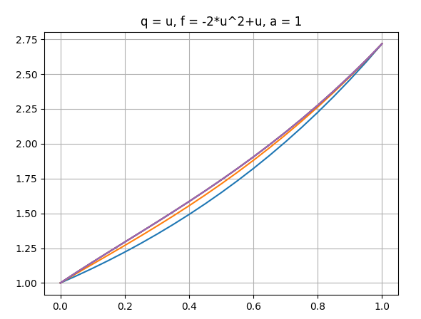
Hello everyone, I am solving the problem of constructing a nonlinear anomalous diffusion equation with the Caputo derivative, using the Grunwald-Letnikov approximation, with zero boundary conditions. I get the following chart. I need to compare with known analytical solution. I am plotting an analytical solution in maple 3d. The question is how can I build the same graph in FEniCS, so that it is clear whether my graph is being built correctly?
from dolfin import *
import matplotlib.pyplot as plt
import numpy as np
import scipy.special
alpha = 1 #Derivative exponent
T = 1 #Maximum time (up to which we calculate u)
M = 10 #Number of intervals in the time grid
dt = T/M #Time step
u0 = Expression('exp(x[0])', degree=4) #Initial condition
mesh = UnitIntervalMesh(20) #Set up a spatial grid
V = FunctionSpace(mesh, 'CG', 4) #We define the space of functions
#Set the boundary conditions
def boundary(x, on_boundary):
return on_boundary
bc = DirichletBC(V, u0, boundary)
#We introduce the functions u and v in order to determine a(u,v) and L(v)
v = TestFunction(V)
ut = [interpolate(Constant(0.0), V) for j in range(M+1)] #The value of the function u at different times
ut[0] = interpolate(u0, V) #initial #Initial condition
#The functions q(u) and f(u) from the problem statement
def q(uk):
return uk
def f(uk):
return -2 * uk**2 + uk
tol = 1.0E-5 #Accuracy at which we stop iterations
maxiter = 50 #The maximum allowable number of iterations (the condition on the number of iterations can be removed in principle)
t = dt #We start the calculations from the first moment in time
while t <= T: #Time cycle
print("t=",t) #Can be removed
j = int(t//dt) #Determine the node number of the time grid
u_k = interpolate(Constant(0.0), V) #Setting the value of u at the zero iteration
L = (ut[0] + (dt**alpha)*f(u_k) - sum( (-1)**k * scipy.special.binom(alpha, k) * (ut[j-k]-ut[0]) for k in range(1, j)) )*v*dx
eps = 1.0 #Error ||u_k-u_k-1||
itern = 0 #Iteration number
while eps > tol and itern < maxiter: #Iterations
itern += 1 #Iteration number
u = TrialFunction(V)
a = u*v*dx + (dt**alpha)*q(u_k)*inner(nabla_grad(u), nabla_grad(v))*dx
u = Function(V)
solve(a == L, u, bc)
#Calculating differences between alternative iterations and observations
diff = u.vector() - u_k.vector()
eps = np.linalg.norm(diff, ord=np.Inf)
u_k.assign(u) #Update the value of u
ut[j].assign(u) #We write the value of u to the array of values of the function u at different points in time
t += dt #move on to the next point in time
print("complete")
#Building a graph
plt.title('q = u, f = -2*u^2+u, a = 1')
plt.grid(True)
plot(ut[0])
plot(ut[1])
plot(ut[M-3])
plot(ut[M-2])
plot(ut[M-1])
#plt.legend(['ut[M-1]'])
plt.show()
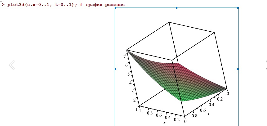
and by the way, an analytical solution is built in maple not with zero boundary conditions, since I could not find the exact solution with zero boundary conditions.