I’m trying to solve the Navier stokes equation in the following domain:

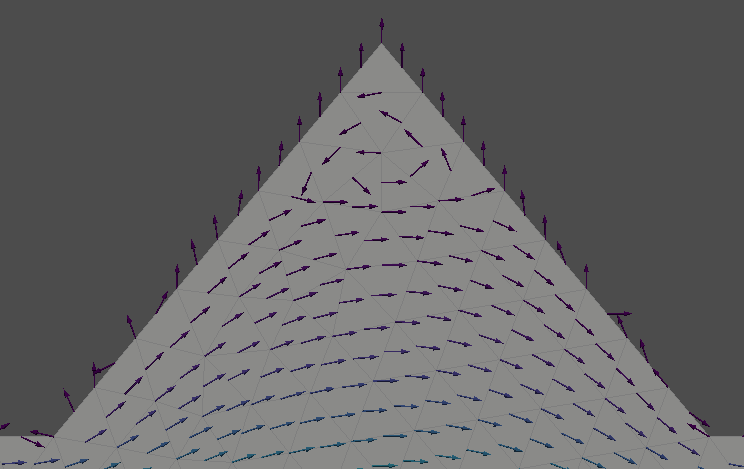
But the solution showed an unexpected behavior along the wall:
For example, in the rectangle region you have a vertical component:
I defined my no slip boundary conditions as
u_nonslip = np.array((0,) * mesh.geometry.dim, dtype=PETSc.ScalarType)
bc_noslip = dirichletbc(u_nonslip, locate_dofs_topological(V, fdim, facet_tags.find(wall_marker)), V)
Appreciate your help and I’m providing the complete code below :
Required modules
import numpy as np
import gmsh
from dolfinx.io.gmshio import model_to_mesh
from mpi4py import MPI

import pyvista
from dolfinx import plot

from ufl import (FacetNormal, FiniteElement, Identity,TestFunction, TrialFunction, VectorElement,
                 div, dot, ds, dx, inner, lhs, nabla_grad, rhs, sym)
from dolfinx.fem import Constant,Function, FunctionSpace, assemble_scalar, dirichletbc, form, locate_dofs_geometrical,locate_dofs_topological
from dolfinx.fem.petsc import assemble_matrix, assemble_vector, apply_lifting, create_vector, set_bc
from dolfinx.io import XDMFFile
from dolfinx.plot import create_vtk_mesh
from petsc4py import PETSc
To generate the geometry
A = np.array([0,0])
B = np.array([5,0])
C = np.array([5,1])
D = np.array([3,1])
E = np.array([2.5,1.6])
F = np.array([2,1])
G = np.array([0,1])


in_flow_marker  = 100
out_flow_marker = 200
wall_marker     = 300

gmsh.initialize()
#gmsh.option.setNumber("General.Terminal",0) #To hide the mesh output values

mesh_size = 0.1
point_1 = gmsh.model.geo.add_point(A[0],A[1], 0, mesh_size)
point_2 = gmsh.model.geo.add_point(B[0],B[1], 0, mesh_size)
point_3 = gmsh.model.geo.add_point(C[0],C[1], 0, mesh_size)
point_4 = gmsh.model.geo.add_point(D[0],D[1], 0, mesh_size)
point_5 = gmsh.model.geo.add_point(E[0],E[1], 0, mesh_size)
point_6 = gmsh.model.geo.add_point(F[0],F[1], 0, mesh_size)
point_7 = gmsh.model.geo.add_point(G[0],G[1], 0, mesh_size)

line_1 = gmsh.model.geo.add_line(point_1, point_2)
line_2 = gmsh.model.geo.add_line(point_2, point_3)
line_3 = gmsh.model.geo.add_line(point_3, point_4)
line_4 = gmsh.model.geo.add_line(point_4, point_5)
line_5 = gmsh.model.geo.add_line(point_5, point_6)
line_6 = gmsh.model.geo.add_line(point_6, point_7)
line_7 = gmsh.model.geo.add_line(point_7, point_1)

curve_loop    = gmsh.model.geo.add_curve_loop([line_1,line_2,line_3,line_4,line_5,line_6,line_7])
plane_surface = gmsh.model.geo.add_plane_surface([curve_loop])

gmsh.model.geo.synchronize()


gmsh.model.addPhysicalGroup(2, [plane_surface], name = "fluid") # You need this for dolfinx


gmsh.model.addPhysicalGroup(1, [line_1,line_3,line_4,line_5,line_6], wall_marker)
gmsh.model.addPhysicalGroup(1, [line_7], in_flow_marker)
gmsh.model.addPhysicalGroup(1, [line_2], out_flow_marker)


gmsh.model.mesh.generate()

mesh, cell_tags, facet_tags = model_to_mesh(gmsh.model, MPI.COMM_WORLD, 0,gdim=2)

gmsh.finalize()
To draw the domain
topology, cell_types, geometry_for_plotting = plot.create_vtk_mesh(mesh, 2)
#If you have the word geometry in place of geometry_for_plotting, it might conflict with the boundingBoxTree statement in the get coordinate function
grid = pyvista.UnstructuredGrid(topology, cell_types, geometry_for_plotting)

pyvista.set_jupyter_backend("pythreejs")

plotter = pyvista.Plotter()
plotter.add_mesh(grid, show_edges=True)
plotter.view_xy()

if not pyvista.OFF_SCREEN:
    plotter.show()
else:
    pyvista.start_xvfb()
    figure = plotter.screenshot("fundamentals_mesh.png")
To solve Navier Stokes equation From the tutorial
t = 0
T = 10
num_steps = 500
dt = T/num_steps

v_cg2 = VectorElement("CG", mesh.ufl_cell(), 2)
s_cg1 = FiniteElement("CG", mesh.ufl_cell(), 1)
V = FunctionSpace(mesh, v_cg2)
Q = FunctionSpace(mesh, s_cg1)

u = TrialFunction(V)
v = TestFunction(V)
p = TrialFunction(Q)
q = TestFunction(Q)
fdim = mesh.topology.dim - 1

class inlet_pressure_class():
    def __init__(self, t):
        self.t = t
    def __call__(self, x):
        return 1 +0*x[0]
inlet_pressure = inlet_pressure_class(t)
u_inlet = Function(Q)
u_inlet.interpolate(inlet_pressure)
bc_inflow = dirichletbc(u_inlet, locate_dofs_topological(Q, fdim, facet_tags.find(in_flow_marker)))


u_nonslip = np.array((0,) * mesh.geometry.dim, dtype=PETSc.ScalarType)
bc_noslip = dirichletbc(u_nonslip, locate_dofs_topological(V, fdim, facet_tags.find(wall_marker)), V)


class outflow_pressure_class():
    def __init__(self, t):
        self.t = t
    def __call__(self, x):
        return 0 +0*x[0]
outlet_pressure = outflow_pressure_class(t)
u_outlet = Function(Q)
u_outlet.interpolate(outlet_pressure)
bc_outflow = dirichletbc(u_outlet, locate_dofs_topological(Q, fdim, facet_tags.find(out_flow_marker)))


bcu = [bc_noslip]
bcp = [bc_inflow, bc_outflow]

u_n = Function(V)
u_n.name = "u_n"
U = 0.5 * (u_n + u)
n = FacetNormal(mesh)
f = Constant(mesh, PETSc.ScalarType((0,0)))
k = Constant(mesh, PETSc.ScalarType(dt))
mu = Constant(mesh, PETSc.ScalarType(1))
rho = Constant(mesh, PETSc.ScalarType(1))

# Define strain-rate tensor
def epsilon(u):
    return sym(nabla_grad(u))

# Define stress tensor
def sigma(u, p):
    return 2*mu*epsilon(u) - p*Identity(u.geometric_dimension())

# Define the variational problem for the first step
p_n = Function(Q)
p_n.name = "p_n"
F1 = rho*dot((u - u_n) / k, v)*dx
F1 += rho*dot(dot(u_n, nabla_grad(u_n)), v)*dx
F1 += inner(sigma(U, p_n), epsilon(v))*dx
F1 += dot(p_n*n, v)*ds - dot(mu*nabla_grad(U)*n, v)*ds
F1 -= dot(f, v)*dx
a1 = form(lhs(F1))
L1 = form(rhs(F1))

A1 = assemble_matrix(a1, bcs=bcu)
A1.assemble()
b1 = create_vector(L1)

# Define variational problem for step 2
u_ = Function(V)
a2 = form(dot(nabla_grad(p), nabla_grad(q))*dx)
L2 = form(dot(nabla_grad(p_n), nabla_grad(q))*dx - (1/k)*div(u_)*q*dx)
A2 = assemble_matrix(a2, bcs=bcp)
A2.assemble()
b2 = create_vector(L2)

# Define variational problem for step 3
p_ = Function(Q)
a3 = form(dot(u, v)*dx)
L3 = form(dot(u_, v)*dx - k*dot(nabla_grad(p_ - p_n), v)*dx)
A3 = assemble_matrix(a3)
A3.assemble()
b3 = create_vector(L3)

# Solver for step 1
solver1 = PETSc.KSP().create(mesh.comm)
solver1.setOperators(A1)
solver1.setType(PETSc.KSP.Type.BCGS)
pc1 = solver1.getPC()
pc1.setType(PETSc.PC.Type.HYPRE)
pc1.setHYPREType("boomeramg")

# Solver for step 2
solver2 = PETSc.KSP().create(mesh.comm)
solver2.setOperators(A2)
solver2.setType(PETSc.KSP.Type.BCGS)
pc2 = solver2.getPC()
pc2.setType(PETSc.PC.Type.HYPRE)
pc2.setHYPREType("boomeramg")

# Solver for step 3
solver3 = PETSc.KSP().create(mesh.comm)
solver3.setOperators(A3)
solver3.setType(PETSc.KSP.Type.CG)
pc3 = solver3.getPC()
pc3.setType(PETSc.PC.Type.SOR)

xdmf = XDMFFile(mesh.comm, "poiseuille.xdmf", "w")
xdmf.write_mesh(mesh)
xdmf.write_function(u_n, t)
xdmf.write_function(p_n, t)

import numpy as np
def u_exact(x):
    values = np.zeros((2, x.shape[1]), dtype=PETSc.ScalarType)
    values[0] = 4*x[1]*(1.0 - x[1])
    return values
u_ex = Function(V)
u_ex.interpolate(u_exact)

L2_error = form(dot(u_ - u_ex, u_ - u_ex)*dx)

for i in range(num_steps):
    # Update current time step
    t += dt

    # Step 1: Tentative veolcity step
    with b1.localForm() as loc_1:
        loc_1.set(0)
    assemble_vector(b1, L1)
    apply_lifting(b1, [a1], [bcu])
    b1.ghostUpdate(addv=PETSc.InsertMode.ADD_VALUES, mode=PETSc.ScatterMode.REVERSE)
    set_bc(b1, bcu)
    solver1.solve(b1, u_.vector)
    u_.x.scatter_forward()

    # Step 2: Pressure corrrection step
    with b2.localForm() as loc_2:
        loc_2.set(0)
    assemble_vector(b2, L2)
    apply_lifting(b2, [a2], [bcp])
    b2.ghostUpdate(addv=PETSc.InsertMode.ADD_VALUES, mode=PETSc.ScatterMode.REVERSE)
    set_bc(b2, bcp)
    solver2.solve(b2, p_.vector)
    p_.x.scatter_forward()

    # Step 3: Velocity correction step
    with b3.localForm() as loc_3:
        loc_3.set(0)
    assemble_vector(b3, L3)
    b3.ghostUpdate(addv=PETSc.InsertMode.ADD_VALUES, mode=PETSc.ScatterMode.REVERSE)
    solver3.solve(b3, u_.vector)
    u_.x.scatter_forward()
    # Update variable with solution form this time step
    u_n.x.array[:] = u_.x.array[:]
    p_n.x.array[:] = p_.x.array[:]

    # Write solutions to file
    xdmf.write_function(u_n, t)
    xdmf.write_function(p_n, t)

    # Compute error at current time-step
    error_L2 = np.sqrt(mesh.comm.allreduce(assemble_scalar(L2_error), op=MPI.SUM))
    error_max = mesh.comm.allreduce(np.max(u_.vector.array - u_ex.vector.array), op=MPI.MAX)
    # Print error only every 20th step and at the last step
#     if (i % 20 == 0) or (i == num_steps - 1):
#         print(f"Time {t:.2f}, L2-error {error_L2:.2e}, Max error {error_max:.2e}")
# # Close xmdf file
xdmf.close()
To plot the solution
pyvista.set_jupyter_backend("pythreejs")
topology, cell_types, geometry = create_vtk_mesh(V)
values = np.zeros((geometry.shape[0], 3), dtype=np.float64)
values[:, :len(u_n)] = u_n.x.array.real.reshape((geometry.shape[0], len(u_n)))

# Create a point cloud of glyphs
function_grid = pyvista.UnstructuredGrid(topology, cell_types, geometry)
function_grid["u"] = values
glyphs = function_grid.glyph(orient="u", scale=False,factor=0.04,clamping=False)


# Create a pyvista-grid for the mesh
grid = pyvista.UnstructuredGrid(*create_vtk_mesh(mesh, mesh.topology.dim))

# Create plotter
plotter = pyvista.Plotter()
# plotter.add_mesh(grid, style="wireframe", color="k")
plotter.add_mesh(grid, show_scalar_bar=True,show_edges=True, opacity=0.5, color="w",
           lighting=True)
plotter.add_mesh(glyphs,show_scalar_bar=True)
plotter.view_xy()
if not pyvista.OFF_SCREEN:
    plotter.show()
else:
    pyvista.start_xvfb()
    fig_as_array = plotter.screenshot("glyphs.png")