When I use dolfin to solver Navier-Stokes equations, no-slip condition was used at the wall, but after sever steps, the error imformation raised. When I used Paraview to open the result files, I find the velocity at wall was not zero. I don’t know what makes this, and here is my code :
import meshio
#import matplotlib.pyplot as pt
from dolfin import *
#msh = meshio.read("import_stl.msh")
msh=meshio.read("msh_nobc.msh")
meshio.write("mesh_nobc.xdmf", meshio.Mesh(points=msh.points, cells={"tetra": msh.cells["tetra"]}))
#boundary face
meshio.write("mf_nobc.xdmf", meshio.Mesh(points=msh.points, cells={"triangle": msh.cells["triangle"]},cell_data={"triangle": {"name_to_read": msh.cell_data["triangle"]["gmsh:physical"]}}))
#boundary cell
meshio.write("cf_nobc.xdmf", meshio.Mesh(points=msh.points, cells={"tetra": msh.cells["tetra"]},cell_data={"tetra": {"name_to_read":msh.cell_data["tetra"]["gmsh:physical"]}}))
mesh = Mesh()
with XDMFFile("mesh_nobc.xdmf") as infile:
    infile.read(mesh)
##
mvc = MeshValueCollection("size_t", mesh, 2)
with XDMFFile("mf_nobc.xdmf") as infile:
    infile.read(mvc, "name_to_read")
mf = cpp.mesh.MeshFunctionSizet(mesh, mvc)
boundary_markers=MeshFunction("size_t",mesh,mvc)
##
mvc = MeshValueCollection("size_t", mesh, 3)
with XDMFFile("cf_nobc.xdmf") as infile:
    infile.read(mvc, "name_to_read")
cf = cpp.mesh.MeshFunctionSizet(mesh, mvc)
T=0.1
splenic_marker=2
smv_marker=1
portal_marker=3
wall_marker=4
domain_marker=5
#deltat=T/num_steps
deltat=0.001
num_steps=100
mu=0.0000035
rho=0.000001060
V=VectorFunctionSpace(mesh,"P",3) #velocity space
Q=FunctionSpace(mesh,"P",1) #pressure space
bcu_smv=DirichletBC(V,Constant((-192.0114,40.6245,74.7075)),boundary_markers,smv_marker)
bcu_splenic=DirichletBC(V,Constant((-61.47694,3.3229,-323.18657)),boundary_markers,splenic_marker)
bcp_portal=DirichletBC(Q,Constant(0.66661),boundary_markers,portal_marker)
bcu_wall=DirichletBC(V,Constant((0,0,0)),boundary_markers,wall_marker)
bcu=[bcu_smv,bcu_splenic,bcu_wall]
bcp=[bcp_portal]
u = TrialFunction(V)
v = TestFunction(V)
p = TrialFunction(Q)
q = TestFunction(Q)

# t=n (u,p) unknown
#u_ = Function(V)
#p_ = Function(Q)

# t=n-1 known
#u_1 = Function(V)
#p_1 = Function(Q)
u0=Function(V)
u1=Function(V)
p1=Function(Q)
#normal
n  = FacetNormal(mesh)
# force
f  = Constant((0, 0,-9810))
###chorin
#step1
#F1 = dot((u-u_1)/deltat,v)*dx+dot(nabla_grad(u_1).T*u_1,v)*dx+(mu/rho)*inner(nabla_grad(u),nabla_grad(v))*dx-dot(f,v)*dx
F1=(1/deltat)*inner(u - u0, v)*dx+inner(dot(nabla_grad(u0),u0),v)*dx+mu/rho*inner(grad(u),grad(v))*dx-inner(f,v)*dx
a1 = lhs(F1)
L1 = rhs(F1)

# step2
a2 = inner(nabla_grad(p),nabla_grad(q))*dx
L2 = -(1/deltat)*div(u1)*q*dx

# step3
a3 = inner(u,v)*dx
L3 = inner(u1,v)*dx-deltat*inner(nabla_grad(p1),v)*dx

# matrix
A1 = assemble(a1)
A2 = assemble(a2)
A3 = assemble(a3)
[bc.apply(A1) for bc in bcu]
[bc.apply(A2) for bc in bcp]
# Use amg preconditioner if available
#prec = "amg" if has_krylov_solver_preconditioner("amg") else "default"

# boundary condition
#[bc.apply(A1) for bc in bcu]
#[bc.apply(A2) for bc in bcp]
#[bc.apply(A3) for bc in bcu]

# output
ufile = File('results/u.pvd')
pfile = File('results/p.pvd')
t=deltat
# Compute tentative velocity step
#while t < T + DOLFIN_EPS:
for n in range(num_steps):
    t+=deltat
    begin("Computing tentative velocity")
    b1 = assemble(L1)
    [bc.apply(b1) for bc in bcu]
    solve(A1, u1.vector(), b1, "gmres", "default")
    end()

    # Pressure correction
    begin("Computing pressure correction")
    b2 = assemble(L2)
    [bc.apply(b2) for bc in bcp]
    solve(A2, p1.vector(), b2, "gmres", "hypre_amg")
    end()

	# Velocity correction
    begin("Computing velocity correction")
    b3 = assemble(L3)
    #[bc.apply(b3) for bc in bcu]
    solve(A3, u1.vector(), b3, "gmres", "jacobi")
    end()

    # Plot solution
    #plot(p1, title="Pressure", rescale=True)
    #plot(u1, title="Velocity", rescale=True)
    #print(p1)
    #print(u1)
	# Save to file
    ufile << u1
    pfile << p1
    #plot(u1)
	# Move to next time step
    u0.assign(u1)

    #t += deltat
    print( "t =", t)
# Hold plot
#interactive()
#pt.plot(mf)
#pt.show()
#ds_custom = Measure("ds", domain=mesh, subdomain_data=mf, subdomain_id=4)
#print(format(assemble(1*ds_custom),".20f"))
The velocity magnitude distribution is like this when t=0.001s, at this time the velocity at wall is still zero(boundary condition at the red region is the pressure-outlet):

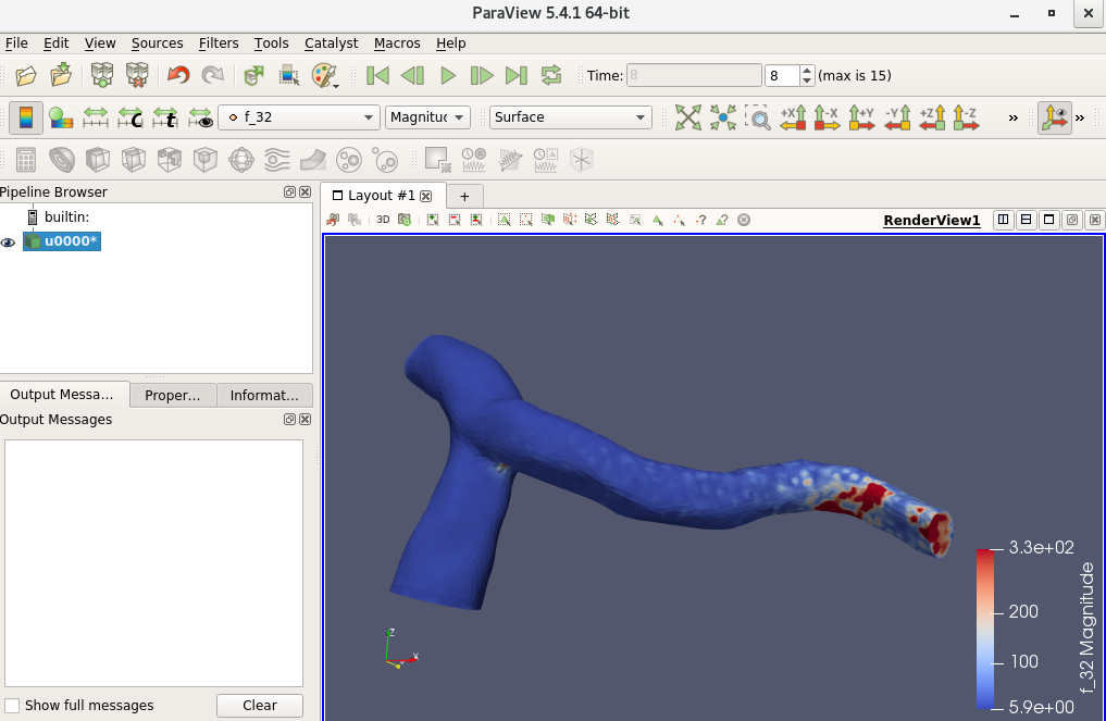
The velocity magnitude distribution is like this when t=0.008s, the velocity at the wall at this time raised:
The error imformation is as belows:
    return cpp.la.solve(A, x, b, method, preconditioner)
RuntimeError:

*** -------------------------------------------------------------------------
*** DOLFIN encountered an error. If you are not able to resolve this issue
*** using the information listed below, you can ask for help at
***
***     fenics-support@googlegroups.com
***
*** Remember to include the error message listed below and, if possible,
*** include a *minimal* running example to reproduce the error.
***
*** -------------------------------------------------------------------------
*** Error:   Unable to solve linear system using PETSc Krylov solver.
*** Reason:  Solution failed to converge in 0 iterations (PETSc reason DIVERGED_NANORINF, residual norm ||r|| = inf).
*** Where:   This error was encountered inside PETScKrylovSolver.cpp.
*** Process: 0
***
*** DOLFIN version: 2019.1.0
*** Git changeset:  2e001bd1aae8e14d758264f77382245e6eed04b0
*** -------------------------------------------------------------------------