Hi,
I am trying to solve a model advection-diffusion problem in Chapter 2 of the book " Finite Element Methods for Flow Problems" by Donea and Huerta.
the system is
with the boundary conditons
u(0) = 0
u(1) = 0
I am using \nu=0.02 and 5 elements for my solution
I have been able to match my solutions when solving the problem with linear elements(p=1). I am unable to get any sensible result when I try to use quadratic (p=2) elements
I basically change the element order by making the function space order from
V = FunctionSpace ( my_mesh, 'CG', 1)
to
V = FunctionSpace ( my_mesh, 'CG', 2)
to get the quadatic mesh
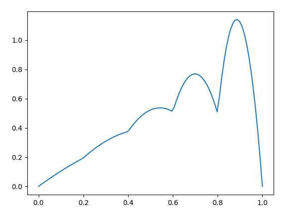
However, when I solve the system and plot the results, I am getting a piecewise linear plot

the actual figure from the source is ( see Pe=5) which is a squiggly solution.

I also tried plotting the nodes, elements, and coordinates for the mesh, but I was surprised to find that they were still 2 noded elements used for the calculation even when the degree was 2 in the FunctionSpace. Since I am using 5 elements, the quadratic 1D mesh should have 11 elements, but I have only 6. (See output after the code)
Could someone guide me on how to get the correct solution?
My code
from __future__ import print_function
from fenics import *
from ufl import nabla_div
import pylab as plt
import numpy as np

## convection_diffusion simulates a 1D convection diffusion problem in Fig 2.1
#    - a*ux - (nu ux),x = f in Omega = the unit interval.
#      u(0) = 0
#      u(1) = 0
#      f=1
my_nu=0.02
n_ele=5
#Define the mesh
my_mesh = UnitIntervalMesh ( n_ele )

#  Set the function space.
V = FunctionSpace ( my_mesh, 'CG', 2)
#  Set the trial and test functions.
#
u = TrialFunction ( V )
v = TestFunction ( V )

#  Set the nu value
mu = Constant ( my_nu )

s = Constant ( 1.0 )
#
#  Define the bilinear form and right hand side
#
aa= Constant ( 1.0 )
a = ( aa* v* u.dx(0) + mu * u.dx(0) * v.dx(0) ) * dx
L = s * v * dx


#  Define the boundary condition.

def boundary ( x ):
   value = x[0] < DOLFIN_EPS or 1.0 - DOLFIN_EPS < x[0]
   return value

bc = DirichletBC ( V, 0, boundary )
#  Solve- use default guess
uh = Function ( V )
#  Solve the system.
solve ( a == L, uh, bc )

#  Plot the solution.
h=1/n_ele
fig = plt.figure (dpi=110 )
ax = plt.subplot ( 111 )
plot (uh, label = 'Computed Pe=%.2f'% (1*h/2/my_nu  ))
ax.legend ( )
ax.grid ( True )
ax.set_ylim([0,1.5])
plt.title ( 'convection_diffusion solutions, # ele %d' % ( n_ele ) )
plt.show()

#  Write NODES, ELEMENTS and VALUES
#
node_num = my_mesh.num_vertices ( )
node_xy = my_mesh.coordinates ( )

print ( "Nodes")
for row in node_xy:
      print(row)


print ( "Elements")

#  Print ELEMENTS array

element_num = my_mesh.num_cells ( )
element_node = my_mesh.cells ( )

for row in element_node:
           print(row)

print ( " Nodal Values")
#  Create a VALUES array, and write it to a file.
#
u_nodal_values = uh.vector ( )
u_array = u_nodal_values.get_local ( )
value_num = my_mesh.num_vertices ( )
node_value = np.zeros ( node_num )

for i in range ( 0, value_num ):
    print(u_array[i] )
Output from Code
Nodes
[ 0.]
[ 0.2]
[ 0.4]
[ 0.6]
[ 0.8]
[ 1.]
Elements
[0 1]
[1 2]
[2 3]
[3 4]
[4 5]
Nodal Values
0.0
0.49944096704
1.12402169232
0.510899864052
0.769494036811
0.374829298033