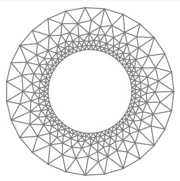
I am using GMSH to produce a sequence of meshes of an annulus (centered at 0, inner radius 1, outer radius 2), with greater resolution on the inner circle to get better accuracy:
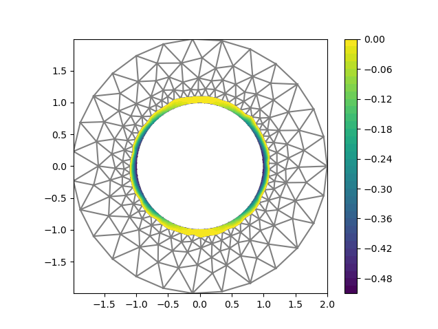
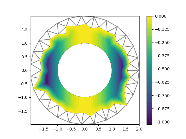
I am solving a poisson equation with exact solution u_ex = 0 if x[0]<=0, x[0]**2 otherwise, Dirichlet BCs on the inner ring, Neumann on the outer ring.
Computing the achieved order of convergence (L2 norm) yields: [ 3.04670631 -0.08825267 2.56832882 2.30941509 1.64144749 0.59804678 2.70940579], which oscillates a lot (the solution is H2 regular). A similar behaviour is obtained with Dirichlet BCs everywhere.
What could be the explanation for this? Is it a problem of the imposition of the boundary conditions?
Thank you in advance…
Let me post the relevant code, mesh generation comes below:
# %% Some data (e.g. exact solution and what not)

# Mesh path
mesh_path = "/home/annulus/"

# Resolutions
resolutions = [0.2, .1, .05, .025, .0125, 0.00625, 0.003125] # mesh width array


# Exact solution and corresponding source
class solution(UserExpression):
    def __init__(self, **kwargs):
        """ Construct the source function """
        super().__init__(self, **kwargs)

    def eval(self, values, x):
        """ Evaluate the source function """
        if x[0] >= 0:
            values[0] = -x[0] ** 2 / 2
        else:
            values[0] = 0


class source(UserExpression):
    def __init__(self, **kwargs):
        """ Construct the source function """
        super().__init__(self, **kwargs)

    def eval(self, values, x):
        """ Evaluate the source function """
        if x[0] >= 0:
            values[0] = 1
        else:
            values[0] = 0


class normal_derivative(UserExpression):
    def __init__(self, **kwargs):
        super().__init__(self, **kwargs)

    def eval(self, values, x):
        if x[0] >= 0:
            if x[0] ** 2 + x[1] ** 2 < 1.5 ** 2:
                values[0] = + x[0]**2
            else:
                values[0] = - x[0]**2 / 2
        else:
            values[0] = 0


u_ex = solution()
f = source()
f_D = solution()  # Dirichlet BC
f_N = normal_derivative() # Neumann BC


# %% Read that mesh

def read_mesh(resolution, mesh_path=mesh_path):
    # The volumetric mesh
    mesh = Mesh()
    with XDMFFile(mesh_path + "mesh_" + str(resolution) + ".xdmf") as infile:
        infile.read(mesh)

    # The boundary conditions
    mvc = MeshValueCollection("size_t", mesh, 1)
    with XDMFFile(mesh_path + "facet_mesh_" + str(resolution) + ".xdmf") as infile:
        infile.read(mvc, "name_to_read")
    mf = MeshFunctionSizet(mesh, mvc)  # remember, tag 3 is inner ring, tag 2 outer ring

    L1 = FiniteElement("Lagrange", mesh.ufl_cell(), 1)
    V = FunctionSpace(mesh, L1)

    return mesh, mf, V


# %% The problem

def solve_single_pb(resolution):

    (mesh, mf, V) = read_mesh(resolution)

    plot(mesh)
    plt.show()

    U = TrialFunction(V)
    v = TestFunction(V)

    # Functional formulation
    dOuterRing = Measure("ds", subdomain_data=mf, subdomain_id=2)

    F = inner(grad(U), grad(v)) * dX - f_N * v * dOuterRing - f * v * dX
    a, L = lhs(F), rhs(F)

    # Boundary conditions
    bcs = [DirichletBC(V, f_D, mf, 3)]  # inner ring, outer ring has already Neumann BCs

    u = Function(V)
    solve(a == L, u, bcs)

    err = errornorm(u_ex, u)

    return err

# %% Error checking

err_vec = []

for res in resolutions:
    err_vec.append(solve_single_pb(res))

err_vec = np.array(err_vec)
ooc = -np.log2( err_vec[1:]/err_vec[:-1])

print(ooc)
And here, the mesh generation code:
# %%
resolution = .0125/8

# An empty geometry
geometry = pygmsh.geo.Geometry()
# Create a model to add data to
model = geometry.__enter__()

# A circle centered at the origin and radius 1
circle = model.add_circle([0.0, 0.0, 0.0], 2.0, mesh_size=5*resolution)  # meshes are always 3D, I will suppress the third component in case

# A hole
hole = model.add_circle([0.0, 0.0, 0.0], 1.0, mesh_size=1*resolution)

# My surface
plane_surface = model.add_plane_surface(circle.curve_loop,[hole.curve_loop])

# Sinchronize, before adding physical entities
model.synchronize()

#%%

# Tagging/marking boundaries and volume.
# Boundaries with the same tag should be added simultaneously
model.add_physical([plane_surface], "volume")
model.add_physical(circle.curve_loop.curves, "outer_ring")
model.add_physical(hole.curve_loop.curves, "inner_ring")

# Generate the mesh
geometry.generate_mesh(dim=2)
geometry.save_geometry(path+"annulus_"+str(resolution)+".geo_unrolled")
gmsh.write(path+"mesh_"+str(resolution)+".msh")
gmsh.clear()
geometry.__exit__()

#%%##########################
# Saving to a better format #
#############################

mesh_from_file = meshio.read(path+"mesh_"+str(resolution)+".msh")

def create_mesh(mesh, cell_type, prune_z = False):
    cells = mesh.get_cells_type(cell_type)  # get the cells of some type: it will change!
    cell_data = mesh.get_cell_data("gmsh:physical", cell_type)
    points = mesh.points[:,:2] if prune_z else mesh.points
    out_mesh = meshio.Mesh(points=points, cells={cell_type: cells}, cell_data={"name_to_read":[cell_data]})
    return out_mesh

# Using the above function, create line and "plane" mesh
line_mesh = create_mesh(mesh_from_file, "line", prune_z=True)
meshio.write(path+"facet_mesh_"+str(resolution)+".xdmf", line_mesh)
triangle_mesh = create_mesh(mesh_from_file, "triangle", prune_z=True)
meshio.write(path+"mesh_"+str(resolution)+".xdmf", triangle_mesh)