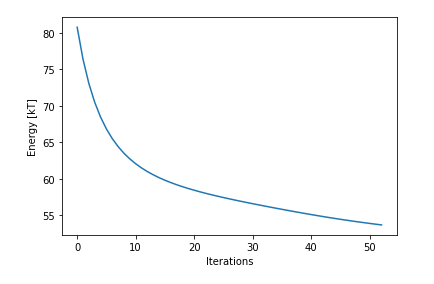
Thank you very much for your response. This is just a section of my code where I am attempting to solve the solve_kozlov() function using different meshes. I am using the initial guess from the previous run. The energy is plotted based on the solution obtained from various iterations. My goal now is to plot the energy as E(r), over the mesh interval, for example, r ranging from 0 to 37.
Here’s my current plot: and the code
import fenics as fe
import matplotlib.pyplot as plt
import numpy as np
import ufl as ufl
from reproject import reproject
def solve_kozlov(mesh, pk, n=2, P_l=np.pi/4, P_r=0.0, D_l=-np.pi/4, D_r=0.0, K_l=np.pi/4, K_r=0.0, l_o=2.1):
def left(x, on_boundary):
return on_boundary and fe.near(x[0], r0)
def right(x, on_boundary):
return on_boundary and fe.near(x[0], rmax)
phiP_element = fe.FiniteElement('CG', mesh.ufl_cell(), n)
ksi_element = fe.FiniteElement('CG', mesh.ufl_cell(), n)
phiD_element = fe.FiniteElement('CG', mesh.ufl_cell(), n)
pk_element = fe.MixedElement([phiP_element, ksi_element, phiD_element])
phiP_space = fe.FunctionSpace(mesh, phiP_element)
ksi_space = fe.FunctionSpace(mesh, ksi_element)
phiD_space = fe.FunctionSpace(mesh, phiD_element)
pk_space = fe.FunctionSpace(mesh, pk_element)
Real_scalar = fe.FunctionSpace(mesh, 'CG', 2)
Real_vector = fe.VectorFunctionSpace(mesh, 'CG', 2)
bc_1 = fe.DirichletBC(pk_space.sub(0), fe.Constant(P_l), left)
bc_2 = fe.DirichletBC(pk_space.sub(0), fe.Constant(P_r), right)
bc_3 = fe.DirichletBC(pk_space.sub(1), fe.Constant(K_l), left)
bc_4 = fe.DirichletBC(pk_space.sub(1), fe.Constant(K_r), right)
bc_5 = fe.DirichletBC(pk_space.sub(2), fe.Constant(D_l), left)
bc_6 = fe.DirichletBC(pk_space.sub(2), fe.Constant(D_r), right)
bcs = [bc_1, bc_2,bc_3,bc_4, bc_5, bc_6]
marker = fe.MeshFunction("size_t", mesh, mesh.topology().dim() - 1, 0)
xa = fe.Expression("x[0]" ,degree=1)
r= fe.interpolate(xa, Real_scalar)
if pk is None:
pk = fe.Function(pk_space)
phiP, ksi, phiD = fe.split(pk)
else:
pk_ = pk
pk = fe.Function(pk_space)
fe.assign(pk, pk_)
phiP, ksi, phiD = fe.split(pk)
vn = fe.TestFunction(pk_space)
dx = fe.Measure("dx", domain=mesh)
K_c = fe.Constant(12.0)
k_o = fe.Constant(0.0)
K_0 = fe.Constant(20.0)
gamma_L = fe.Constant(0.0)
del_P = fe.Constant(0.0)
r_p = r + delta * fe.sin(ksi)
r_d = r - delta * fe.sin(ksi)
integrand1 = (1 + (float(delta) *fe.cos(ksi) *fe.Dx(ksi, 0))) *2 * np.pi * r_p *(1 / fe.cos(ksi)) * ((K_c/2)* (((fe.cos(phiP + ksi)+ fe.cos(phiP - ksi))/2)* fe.Dx(phiP + ksi, 0) * ((1 + (delta * fe.cos(ksi) * fe.Dx(ksi,0))) ** (-1)) + (fe.sin(phiP + ksi)/r_p) - k_o) ** 2 - (k_o ** 2))
integrand2 = (K_0 / 2) * np.pi * r_p * (1 - fe.cos(2 * phiP)) * (1/fe.cos(ksi))* (1 + (float(delta) *fe.cos(ksi) *fe.Dx(ksi, 0)))
integrand3 = gamma_L * 2 * np.pi * r_p * (1/fe.cos(ksi)) *(1 + (float(delta) * fe.cos(ksi) *fe.Dx(ksi, 0)))
integrand4 = del_P * fe.pi * (r_p * r_p) * fe.tan(ksi) * (1 + (float(delta) * fe.cos(ksi) *fe.Dx(ksi, 0)))
integrand9 = - (l_o * fe.tan(ksi)) #* (1 + (float(delta) *fe.cos(ksi) *fe.Dx(ksi,0)))
integrand5 = (
(1 - (float(delta) *fe.cos(ksi) *fe.Dx(ksi, 0))) *2 * np.pi * r_d
* (1 / fe.cos(ksi)) * ((K_c / 2) * (
((fe.cos(phiD + ksi) + fe.cos(phiD - ksi)) / 2) * (-1)
* fe.Dx(phiD + ksi, 0) * ((1 - (delta * fe.cos(ksi) * fe.Dx(ksi, 0))) ** (-1))
+ (fe.sin(-phiD - ksi)/r_d) - k_o
) ** 2 - (k_o ** 2))
)
integrand6 = (K_0 / 2) * np.pi * r_d * (1 - fe.cos(2 * phiD)) * (1 / fe.cos(ksi))* (1 - (float(delta) *fe.cos(ksi) *fe.Dx(ksi, 0)))
integrand7 = gamma_L * 2 * np.pi * r_d * (1 / fe.cos(ksi)) *(1 - (float(delta) * fe.cos(ksi) * fe.Dx(ksi, 0)))
integrand8 = del_P * fe.pi * (r_d * r_d) * fe.tan(-ksi) * (1 - (float(delta) * fe.cos(ksi) * fe.Dx(ksi, 0)))
integrand10 = - (l_o * fe.tan(-ksi)) * (1 - (float(delta) * fe.cos(ksi) *fe.Dx(ksi, 0)))
functional = (
integrand1 * dx + integrand2 * dx + integrand3 * dx + integrand4 * dx
+ integrand5 * dx + integrand6 * dx + integrand7 * dx
+ integrand8 * dx + integrand9 * dx
)
Integ1=functional-integrand9*dx
Integ=functional
weak_form = fe.derivative(Integ , pk, fe.TestFunction(pk_space))
jacobian = fe.derivative(weak_form, pk, fe.TrialFunction(pk_space))
problem = fe.NonlinearVariationalProblem(weak_form, pk, bcs, jacobian)
solver = fe.NonlinearVariationalSolver(problem)
solver.parameters["newton_solver"]["maximum_iterations"]=50
solver.parameters["newton_solver"]["relative_tolerance"]=1e-15
solver.solve()
Energy= fe.assemble(Integ1)
print('Energy=', Energy)
return pk, Integ1
delta = fe.Constant(1.2)
r0 = delta * fe.sin(np.pi / 4)
rmax = 37.0
mesh = fe.IntervalMesh(9, r0, rmax)
pk=None
pk_initial, Integ1 = solve_kozlov(mesh, pk)
with fe.XDMFFile('solution0.xdmf') as xdmf:
xdmf.write(pk_initial)
num_of_nodes = list(range(10, 66))
integral_values = []
for i in range(0, 53):
new_mesh = fe.IntervalMesh(num_of_nodes[i], r0, rmax)
pk_initial_new = reproject(pk_initial.split(True), mesh, new_mesh)
pk_initial, Integ1 = solve_kozlov(new_mesh, pk_initial_new)
with fe.XDMFFile(f'solution{i}.xdmf') as xdmf:
xdmf.write(pk_initial)
mesh = fe.Mesh(new_mesh)
integral_value = fe.assemble(Integ1)
integral_values.append(integral_value)
plt.plot(integral_values)
plt.xlabel('iterations')
plt.ylabel('Energy')
plt.show()
print('integral values=', integral_value)
# So here comes the problem how to make new plot?
step = 0.1
xi = np.arange(r0, rmax, step)
yi = np.zeros(len(xi))
print(len(xi), len(yi), len(integral_values))
for i in range(0, len(xi)):
pk, Integ1 = solve_kozlov(new_mesh, pk_initial_new)
yi[i] = integral_values(xi[i])
plt.plot(xi, yi)
plt.xlabel('r')
plt.ylabel('Energy')
plt.show()