Can an array of values be assigned to the source term?

[fea]

I want to solve Poisson’s Equation where the forcing term is provided as an array of values rather than one constant or a function like in the tutorial examples. Is there a way to do this? Or am I required to interpolate a function from the array of forcing values?

My code is below:

# Create mesh
domain = df.mesh.create_unit_square(MPI.COMM_WORLD,20,20)
tdim = domain.topology.dim 
fdim = domain.topology.dim-1 
domain.topology.create_connectivity(fdim, tdim)

# Create functionspace
V = df.fem.functionspace(mesh = domain, element = ("Lagrange",1))

# Define Trial and Test functions
u = ufl.TrialFunction(V)
s = ufl.TestFunction(V)

# Define forcing term
vals = np.float64(np.random.uniform(200,300,size = (20,20)))
f = df.fem.Constant(domain = domain, c = vals) # This compiles

# Abstract form of variational problem
L = f*s*ufl.dx # This does not compile and raises a ValueError 

The last line raises the error:

ValueError: Can only integrate scalar expressions. The integrand is a tensor expression with value shape (20, 20) and free indices with labels ().

I’m adding the ufl tag because this might be ufl related rather than due to dolfinx.

[nate]

Stochastic coefficients are pretty complicated to implement “correctly” in terms of assuring a sample approximation discretised in space satisfies sufficient regularity.

Ignoring this warning, maybe try the following:

DG0 = df.fem.functionspace(domain, ("DG", 0))
f = df.fem.Function(DG0)
f_size_local = DG0.dofmap.index_map.size_local
f.x.array[:f_size_local] = np.random.uniform(200, 300, size=f_size_local)
f.x.scatter_forward()

This gives you a piecewise constant random value of f defined in each cell.

f will look something like this:

Going back to my warning: bear in mind that as you refine the mesh the characteristics of your sample approximation will be very different because of the finer spatial resolution.

[fea]

The line compiled, so that’s a step in the right direction. However, I’m not familiar with using the Discontinuous Galerkin function space, and it looks like working with this function space has its own quirks that the Lagrangian one I’m more familiar with does not. I only started using Fenics a few weeks ago.

Going with this function space instead, running the lines of code to locate the degrees of freedom necessary for defining the boundary conditions

boundary_facets = df.mesh.exterior_facet_indices(domain.topology)
boundary_dofs = df.fem.locate_dofs_topological(V = DG0, entity_dim=1, entities= boundary_facets)

yields an empty array. That’s the immediate issue I noticed, however after fixing this, there might be others running the rest of my code:

# Define BC given boundary_dofs
uD = df.fem.dirichletbc(df.default_scalar_type(0),boundary_dofs,DG0)

# Define Trial and Test functions
u = ufl.TrialFunction(DG0)
s = ufl.TestFunction(DG0)

# Abstract form of variational problem
## a(u,s)
a = ufl.dot(ufl.grad(u),ufl.grad(s)) * ufl.dx
## L(s)
L = f*s*ufl.dx

# define problem
from dolfinx.fem.petsc import LinearProblem
problem = LinearProblem(a=a,L=L,bcs = [uD]) 

# solve
uh = problem.solve()

# Plot
u_topology, u_cell_types, u_geometry = df.plot.vtk_mesh(DG0.mesh)
u_grid = pv.UnstructuredGrid(u_topology, u_cell_types, u_geometry)
u_grid.point_data["u"] = uh.x.array.real
warped = u_grid.warp_by_scalar("u", factor=0.2) # 3D warping of solution 
u_grid.set_active_scalars("u")
u_plotter = pv.Plotter()
u_plotter.add_mesh(warped, show_edges=True)
u_plotter.show()

All of the above code ran just fine with a Lagrangian function space for other problems, but might not using this function space.

[Stein]

I don’t think @nate means for you to use DG for the solution and trial space, only for interpolating your forcing function.

@fea

I want to solve Poisson’s Equation where the forcing term is provided as an array of values rather than one constant or a function like in the tutorial examples.

But what do you actually mean by that? The Poisson equation is defined as mapping the laplacian of your solution to a function… It has no meaning when the right hand side is an array of values.

So one way or another, you have to translate your “array of values” to a function, through interpolation of some sorts. @nate’s example interpolates onto a very non-restrictive space (DG).

[fea]

I’m sorry, I misread your post and hastily typed out a reply earlier. So, we want to use a separate function space to interpolate our sources to to create a function, and a different function space for the test and trial functions. This is similar to what was done in an older example I found here where f and g and the test and trial function each have their own respective function spaces.

Also, to your confusion, my true problem is one such that I have a dataset in which I don’t know what the symbolic or analytic definition of the data is, and I needed to know how to handle this. I think you answered that as well by saying that I need to interpolate this data which is exactly what Nate’s code did.

Making the necessary changes to my code, this did work… I think? Let me know what you think.

# Create mesh
domain = df.mesh.create_unit_square(MPI.COMM_WORLD,20,20)
tdim = domain.topology.dim 
fdim = domain.topology.dim-1 
domain.topology.create_connectivity(fdim, tdim)

# Create functionspace for Test and Trial functions
V = df.fem.functionspace(mesh = domain, element = ("Lagrange",1))
# Define Trial and Test functions
u = ufl.TrialFunction(V)
s = ufl.TestFunction(V)

# Create separate functionspace for forcing term
DG0 = df.fem.functionspace(domain, ("DG", 0))
# Define forcing function
f = df.fem.Function(DG0)
f_size_local = DG0.dofmap.index_map.size_local
f.x.array[:f_size_local] = np.random.uniform(-100, 100, size=f_size_local)
f.x.scatter_forward()

# Define boundary 
boundary_facets = df.mesh.exterior_facet_indices(domain.topology)
boundary_dofs = df.fem.locate_dofs_topological(V = V, entity_dim=1, entities= boundary_facets)
# Define BC given boundary_dofs
uD = df.fem.dirichletbc(df.default_scalar_type(0),boundary_dofs,V)

# Abstract form of variational problem
## a(u,s)
a = ufl.dot(ufl.grad(u),ufl.grad(s)) * ufl.dx
## L(s)
L = f*s*ufl.dx

# define problem
from dolfinx.fem.petsc import LinearProblem
problem = LinearProblem(a=a,L=L,bcs = [uD]) 
# solve
uh = problem.solve()

# Plot
u_topology, u_cell_types, u_geometry = df.plot.vtk_mesh(V.mesh)
u_grid = pv.UnstructuredGrid(u_topology, u_cell_types, u_geometry)
u_grid.point_data["u"] = uh.x.array.real
warped = u_grid.warp_by_scalar("u", factor=1) # 3D warping of solution 
u_grid.set_active_scalars("u")
u_plotter = pv.Plotter()
u_plotter.add_mesh(warped, show_edges=True)
u_plotter.show()

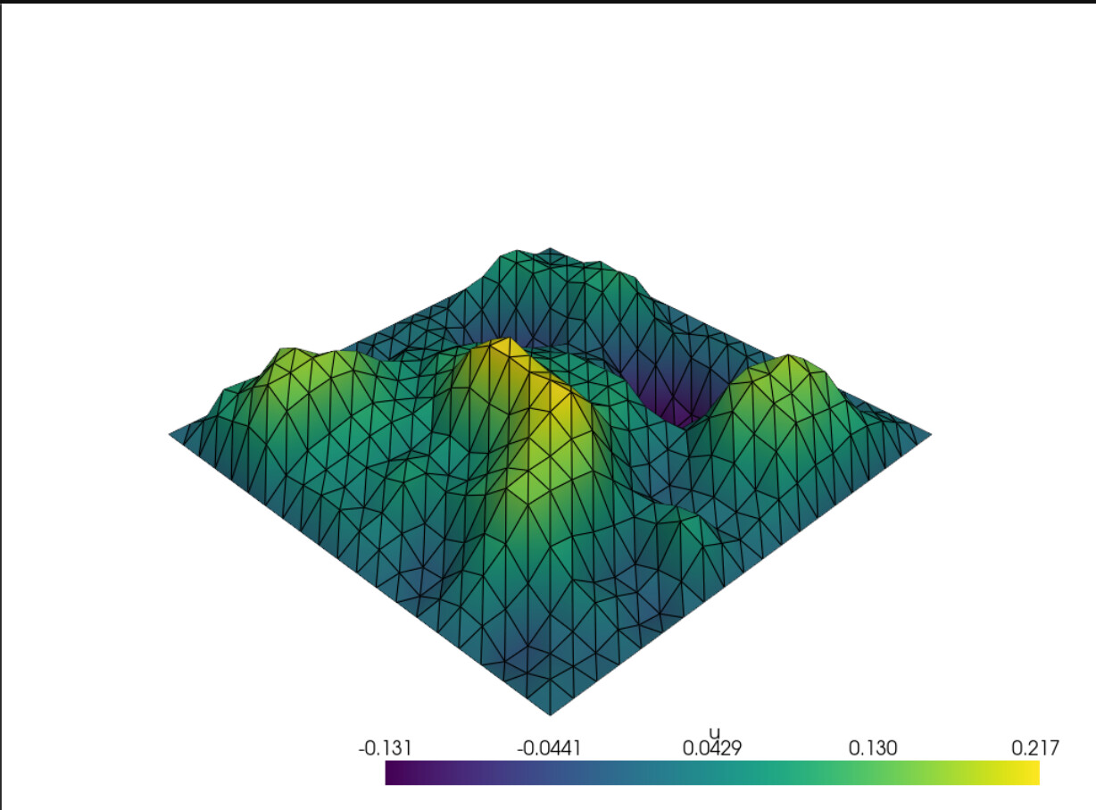
Notice how I changed the line defining populating random values into f to

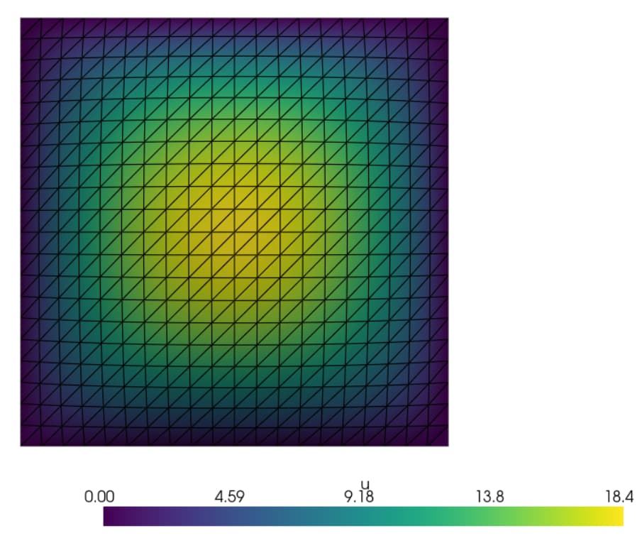
f.x.array[:f_size_local] = np.random.uniform(-100, 100, size=f_size_local) so that the low and high values of the randomizer to be equal and opposite sign. When the distribution of values are a bit more symmetric about 0, I notice I get a random distribution of relative maxima and minima, which I think is what I should expect for a random distribution of sources. However, when I played around with the bounds, I noticed that the more skewed the bounds were away from 0, I would get a larger, smoother, more centered Gaussian hump. Running the original line

f.x.array[:f_size_local] = np.random.uniform(200, 300, size=f_size_local)

(where both bounds are positive), I get

I think that regardless of the bounds, I should expect a random bumpier distribution of multiple relative maxima and minima like the first plot given a random distribution of sources, not a singular smooth centered hump.

[fea]

I just realized that by omitting the motivation for my question, and providing a numpy array using the random number generation, I might have caused a misunderstanding and made you think that I was dealing with a random distribution of values for my PDE, and that this was in the realm of probability, hence bringing up the “Stochastic” terminology. I used numpy’s random number generator to somewhat lazily simulate a distribution of values that I didn’t know the analytic or symbolic definition for. The real distribution of values that I’m working with isn’t quite as random or erratic. I apologize for the confusion on that.

[Stein]

I don’t have access to my laptop right now, but I think what you are seeing is explained as follows:

The Poisson equation is linear, so you can separate the solution into the linear combination of the solution of various linearly combined sources.

Your second plot is this the result of a “constant” force of 250, plus a fluctuating force between -50 and 50. The latter produces a solutuion a factor half of your former plot. That would be 1% the magnitude.

So I’m guessing you simply don’t see the fluctuations in your last plot, but they a there there.

[fea]

A few follow-up questions:

1. Do you know if there is a way to visualize these fluctuations?
2. Is there a way to visualize, f? The shape doesn’t match the domain, so the code I used to plot uh will not work for f.
3. It looks like f_size_local gives the total number of points in the function space, is there a reason why this doesn’t match up with the total number of points that make up the domain which the function space was mapped on to i.e. 20x20 = 400 points?
4. What should I do if the data that I’m populating into f doesn’t fill in all the points which make up f’s function space? I have 20x20 points of source data, but this isn’t enough to fill in all the points making up this discontinuous function space? If I’m not able to fill all of the points, will this lead to inaccuracies in the result?

The latter 2 questions likely stem from a misunderstanding of the nature of discontinuous spaces, I have not used one before. Hopefully these questions aren’t too demanding, I’d hate to waste your time.

[Stein]

2.:
I’d recommend using pyvista4dolfinx (Pyvista4dolfinx). Then simply:

import pyvista4dolfinx as p4d
p4d.plot(f, show=True)

1.:
To confirm my hypothesis? I’d compute a second uh with that constant body force, and substract the results. Below your lines of code:

# Second computation
f.x.array[:] = 250
problem2 = LinearProblem(a=a,L=L,bcs = [uD]) 
uh_250_dif = problem2.solve()
uh_250_dif.name = 'diff'
uh_250_dif.x.array[:] -= uh.x.array[:]

# Plot
import pyvista4dolfinx as p4d
plotter = p4d.Plotter(shape=(1, 2))
p4d.plot(uh, plotter=plotter, subplot=(0,0))
p4d.plot(uh_250_dif, plotter=plotter, subplot=(0,1), show=True)

3.:
f_size_local is the number of degrees of freedom being worked on by the current process. If you run on 1 core, it will simply be the number of dofs of the space. For a DG0 space, this is 1 dof per element. You have a mesh of 20x20x2 elements (x2 because triangles), so 800 dofs.

4.: That’s a good question, and I guess your main challenge. I don’t have a good answer for you. I would honestly not simply assign values to dofs of a DG space, but somehow try to actually interpolate the data that you have to change it from discrete to continuous. But the strategy for operating on an array of measurement data is not really related to FEniCs. If the array is structured in x and y, then I believe numpy has some functionality for interpolating between datapoints. Once you have some representation of your data that can be querried at all (x,y), then you can simply use the f.interpolate functionality of fenics (Interpolation and IO — DOLFINx 0.9.0 documentation)

[nate]

I’m a bit lost in this conversation now. But here’s an example that would use scipy to create a linear interpolation of arbitrary data and then interpolating that interpolation in a FE space…

import dolfinx
from mpi4py import MPI
import scipy.spatial
import scipy.interpolate
import numpy as np
import ufl

if MPI.COMM_WORLD.size > 1:
	raise NotImplementedError("Parallel computation would require preprocessing the source term")


# Data can be anything, but geometry should generate a triangulation which envelops
# the computational domain
data_x = np.mgrid[0:1:5j, 0:1:5j]
data_x = data_x.reshape((2, -1)).T
data_v = data_x[:, 0]**2 + data_x[:, 1]**2  # Make up some data for each point

# The data here is arranged in a structured grid; however, we use a triangulation such
# that this generalises to arbitrary data geometry within the computational domain.
triangle = scipy.spatial.Delaunay(data_x)

# Several numerical schemes for interpolation of the data available
interp = scipy.interpolate.LinearNDInterpolator(triangle, data_v)


# Now back to DOLFINx
mesh = dolfinx.mesh.create_unit_square(MPI.COMM_WORLD, 32, 32)
V = dolfinx.fem.functionspace(mesh, ("CG", 1))
u, v = ufl.TrialFunction(V), ufl.TestFunction(V)


Vf = dolfinx.fem.functionspace(mesh, ("CG", 1))  # This is not restricted to CG space
f = dolfinx.fem.Function(Vf)
f.interpolate(lambda x: interp(x.T[:, :2]))


a = ufl.inner(ufl.grad(u), ufl.grad(v)) * ufl.dx
L = ufl.inner(f, v) * ufl.dx

mesh.topology.create_connectivity(mesh.topology.dim - 1, mesh.topology.dim)
boundary_facets = dolfinx.mesh.exterior_facet_indices(mesh.topology)
boundary_dofs = dolfinx.fem.locate_dofs_topological(V, mesh.topology.dim - 1, boundary_facets)
uD = dolfinx.fem.dirichletbc(dolfinx.default_scalar_type(0), boundary_dofs, V)

from dolfinx.fem.petsc import LinearProblem
problem = LinearProblem(a, L, 
	bcs=[uD],
    petsc_options_prefix="example_problem_",
    petsc_options={"ksp_type": "preonly", "pc_type": "lu"})
uh = problem.solve()[0]

The forcing function in this case:

and the approximate solution:

[fea]

1. Well that’s certainly a convenient package for visualization. I’ll have to give that a try to save some lines of code.
2. I’ll have to give that a try as well. I’m only doing this to make absolutely certain that dolfinx and/or ufl is working properly and I didn’t make a mistake somewhere
3. Ohhhhh okay that makes sense. It’s 2 triangles per cell.
4. So in the end, I likely will have to use an algorithm to come up with an approximated functional definition. Okay. Hopefully what I come up with isn’t too inaccurate, The new challenge will be to make the functional representation as accurate as possible. I do also have an older version of Matlab on my system, so I can try reading in the data into that and see if the result is more accurate or not.

@Stein

But the strategy for operating on an array of measurement data is not really related to FEniCs

Is that right? Over on the scicomp stackexchange, they recommended this and dealii (if I used C) for my use case. They must have assumed that I knew a functional definition for my data beforehand. Thank you for making this clear to me!

[fea]

Yeah, that looks about right! This will provide a useful skeleton for what I will need to do next. Thank you, Nate!

[dokken]

@fea

Is that right? Over on the scicomp stackexchange, they recommended this and dealii (if I used C) for my use case. They must have assumed that I knew a functional definition for my data beforehand. Thank you for making this clear to me!

I think what he means is that at some point you, the user has to decide how you want to transfer your measurement data into a suitable finite element space. This can be a continuous space, a discontinuous space, or just evaluation at the quadrature points used in your FEM formulation.

What Nate shows is one choice of transferring data from measurements to something that can be evaluated by the interpolate function in FEniCS. There are many other choices that can me made as well (Mapping 2D numpy array into dolfinx function - #4 by dokken)

For instance, if your data is voxel based, one could use

Assigning values to function: order issues

Consider something like the following code: from mpi4py import MPI import numpy as np import ufl from dolfinx import fem, mesh, io L = 2 W= 3 nx = 3 ny = 5 nz = 7 msh = mesh.create_box(comm=MPI.COMM_WORLD, points=((0.0, 0.0, 0.), (L, L, W)), n=(nx-1, ny-1, nz-1), cell_type=mesh.CellType.hexahedron,) dx, dy, dz = L/(nx-1), L/(ny-1), W/(nz-1) values = np.arange(nx*ny*nz).reshape(nx, ny, nz) P1 = ufl.FiniteElement("Lagrange", msh.ufl_cell(…

[fea]

Just as a disclaimer: I don’t have a formal education in discrete mathematics or numerical analysis, the most I’ve done in this area is use the finite element method known as the implicit Euler to discretize Poisson’s Equation (as well as the basic direct solvers like the Gauss-Seidal and SOR and their associated stability analyses). So, some of the vocabulary you’re using is a bit unfamiliar to me.

@dokken

or just evaluation at the quadrature points used in your FEM formulation

What are quadrature points?

[dokken]

When we want to evaluate any integral on a computer, this comes down to choosing a quadrature rule for each element, such that we either exactly integrate the function or approximate it to some order.

I have written out the full transformation at

The UFL forms — FEniCS Workshop

In DOLFINx, you have the notion of a quadrature space, which is a space to store data in (at quadrature points), which doesn’t have any underlying basis function, meaning that it cannot be evaluate at any other point that the quadrature points.

See for instance Visualizing quadrature functions as point clouds — scifem