Error increasing with decreasing mesh size

neha · June 17, 2025, 6:49pm

Hi,
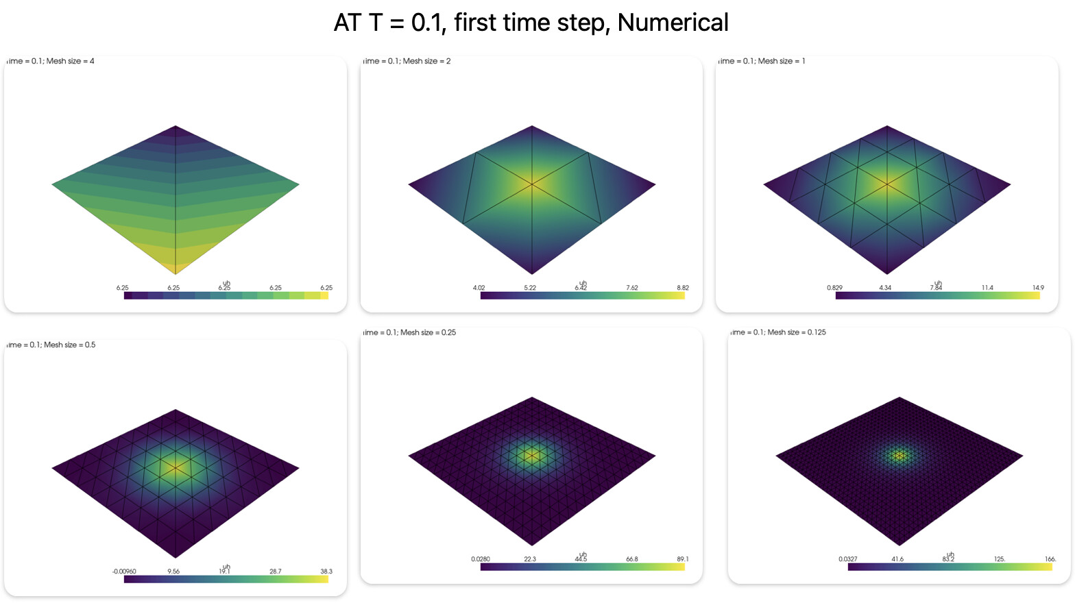
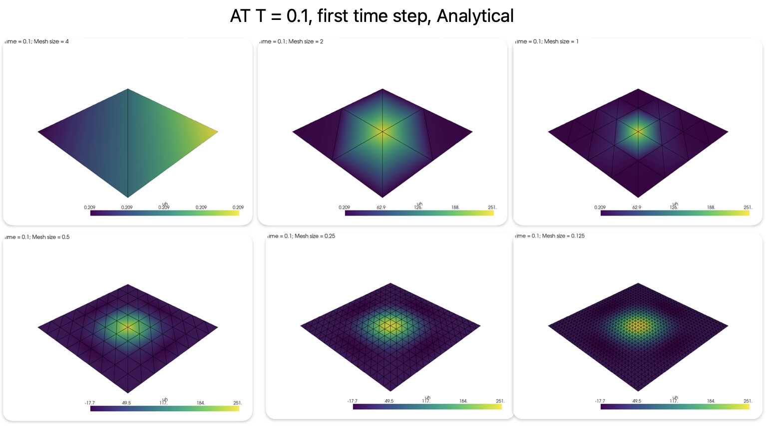
I am working on error convergence analysis for an diffusion example in 2D : Cube is the domain and initial condition is a point source at the centre. Below is the formulation and analytical solution. I am approximating point source as Gaussian function.

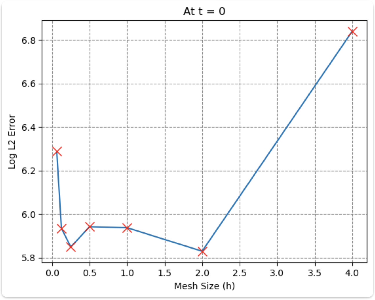
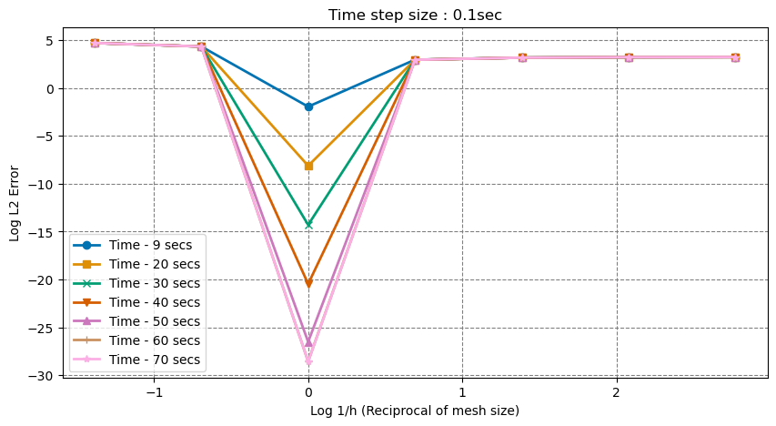
But the L2 error is increasing as I decrease the mesh size, can’t seem to find why this is happening. Tried changing the time w.r.t mesh size, but it didn’t work.

Here is the code:

import matplotlib as mpl
import pyvista
import ufl
import numpy as np

from petsc4py import PETSc
from mpi4py import MPI

from dolfinx import fem, mesh, io, plot
from dolfinx.fem.petsc import assemble_vector, assemble_matrix, create_vector, apply_lifting, set_bc

from dolfinx.fem import (Expression, Function, functionspace,
                         assemble_scalar, dirichletbc, form, locate_dofs_topological)
class exact_solution():
   
    def __init__(self, t, cnt, dim, S0 =100):
 
        self.S0 = S0
        self.t = t
        self.cnt = cnt
        self.dim = dim

    def __call__(self, x):
        sol_approx = 0
        for i in range(self.cnt):
            for j in range(self.cnt):
                norm_factor = (2 if i > 0 else 1) * (2 if j > 0 else 1) ## Normalization factor for the Fourier series terms
                lambda2 = ((np.pi**2) * (i**2 +  j**2))/16 ## Eigenvalue for the Fourier series terms
                sol_approx += (self.S0/16) * norm_factor * np.cos(i*np.pi*x[0]/4) * np.cos(j*np.pi*x[1]/4) * np.exp(-lambda2 * self.t) ## Fourier series term
        return sol_approx

class heat_eq_2D():
    def __init__(self, domain, strt_t, end_t, num_steps,cnt,uexact,u_D,sigma):
        self.domain = domain
        self.V = fem.functionspace(domain, ("Lagrange", 1))
        self.dt = end_t / num_steps
        self.t = strt_t
        self.cnt = cnt
        self.uexact = uexact
        self.u_D = u_D
        self.num_steps = num_steps
        self.sigma = sigma

    def initial_condition(self, x,scale=1,S0=100):
        return scale*S0*np.exp(-0.5*(x[0]**2 + x[1]**2)/(self.sigma**2) )/(2*np.pi*self.sigma**2)
        
    def scale_est(self):
        u_n0 = fem.Function(self.V)
        u_n0.interpolate(lambda x: self.initial_condition(x,S0 = 1))

        dx = ufl.dx(domain=self.domain)
        inital_condt_form = u_n0*dx
        integral = self.domain.comm.allreduce(fem.assemble_scalar(fem.form(inital_condt_form)), op=MPI.SUM)

        self.scale = 1/integral
        # print("Scale factor: ", self.scale)
    
    def error_L2(self, uh, u_ex, degree_raise=3):
        # Create higher order function space
        degree = uh.function_space.ufl_element().degree
        family = uh.function_space.ufl_element().family_name
        mesh = uh.function_space.mesh
        W = functionspace(mesh, (family, degree + degree_raise))
        # Interpolate approximate solution
        u_W = Function(W)
        u_W.interpolate(uh)

        # Interpolate exact solution, special handling if exact solution
        # is a ufl expression or a python lambda function
        u_ex_W = Function(W)
        u_ex_W.interpolate(u_ex)

        # Compute the error in the higher order function space
        e_W = Function(W)
        e_W.x.array[:] = u_W.x.array - u_ex_W.x.array

        # Integrate the error
        error = form(ufl.inner(e_W, e_W) * ufl.dx)
        error_local = assemble_scalar(error)
        error_global = mesh.comm.allreduce(error_local, op=MPI.SUM)
        
        return np.sqrt(error_global)

    def solve_pde(self): 
        self.scale_est()   
        u_n = fem.Function(self.V)
        u_n.name = "u_n"
        u_n.interpolate(lambda x: self.initial_condition(x, scale = self.scale))

        dx = ufl.dx(domain=self.domain)
        inital_condt_form = u_n*dx
        integral = self.domain.comm.allreduce(fem.assemble_scalar(fem.form(inital_condt_form)), op=MPI.SUM)
        # print(f"Integral of initial condition: {integral}")

        # Define solution variable, and interpolate initial solution for visualization in Paraview
        uh = fem.Function(self.V)
        uh.name = "uh"
        uh.interpolate(lambda x: self.initial_condition(x, scale=self.scale))

        u, v = ufl.TrialFunction(self.V), ufl.TestFunction(self.V)
        a = u * v * ufl.dx + self.dt * ufl.dot(ufl.grad(u), ufl.grad(v)) * ufl.dx
        L = u_n  * v * ufl.dx

        bilinear_form = fem.form(a)
        linear_form = fem.form(L)

        A = assemble_matrix(bilinear_form)
        A.assemble()
        b = create_vector(linear_form)

        solver = PETSc.KSP().create(self.domain.comm)
        solver.setOperators(A)
        solver.setType(PETSc.KSP.Type.PREONLY)
        solver.getPC().setType(PETSc.PC.Type.LU)

        time_ls = []
        error_L2_ls = []
        # error_max_ls = []
        for i in range(self.num_steps):
            self.t += self.dt
            self.uexact.t += self.dt
            self.u_D.interpolate(self.uexact)
            
            # Update the right hand side reusing the initial vector
            with b.localForm() as loc_b:
                loc_b.set(0)
            assemble_vector(b, linear_form)

            # Solve linear problem
            solver.solve(b, uh.x.petsc_vec)
            uh.x.scatter_forward()

            # Compute L2 error and error at nodes
            # V_ex = fem.functionspace(self.domain, ("Lagrange", 1))
            # u_ex = fem.Function(V_ex)
            # u_ex.interpolate(self.uexact)
            # error_L2 = np.sqrt(domain.comm.allreduce(fem.assemble_scalar(fem.form((uh - u_ex)**2 * ufl.dx)),
            #                                           op=MPI.SUM))
    
            error_L2_ls.append(self.error_L2(uh,self.uexact))
            time_ls.append(self.t)
            # # Compute values at mesh vertices
            # error_max = self.domain.comm.allreduce(np.max(np.abs(uh.x.array - self.u_D.x.array)), op=MPI.MAX)
            # error_max_ls.append(error_max)

            # Update solution at previous time step (u_n)

            u_n.x.array[:] = uh.x.array
        
        # self.end_num_sol = uh.x.array
        # self.end_ana_sol = u_ex.x.array
        
        # return error_L2_ls, error_max_ls
        return error_L2_ls,time_ls

# Define temporal parameters
t = 0  # Start time
T = 2*60  # Final time

L2_error_dict_master = {}
for dt in [1,0.5,0.1,0.01,0.001]:
    L2_error_dict = {}
    for h in [1,0.8,0.5,0.25]:
        print(f"Solving for mesh size = {h}")
        
        num_steps = int(T/dt)

        # Define mesh
        nx, ny = int(4/h), int(4/h)  # Number of elements in x and y directions
        domain = mesh.create_rectangle(MPI.COMM_WORLD, [np.array([-2, -2]), np.array([2, 2])],
                                    [nx, ny], mesh.CellType.triangle)
        V = fem.functionspace(domain, ("Lagrange", 1))

        u_exact = exact_solution(0,cnt = 5)
        u_D = fem.Function(V)
        u_D.interpolate(u_exact)

        pde_sol_obj = heat_eq_2D(domain, strt_t=0, end_t=T, num_steps=num_steps,
                                cnt=5, uexact=u_exact, u_D=u_D, sigma=h)
        L2_error_dict[h] = pde_sol_obj.solve_pde()
    L2_error_dict_master[dt] = L2_error_dict

dokken · June 22, 2025, 7:10pm

Have you looked at how the solution looks like at after:

Adding the initial condition, i.e.

what is the error norm of the initial condition when you refine the mesh?

Secondly, how does the solution look like visually (after 1 time step, compared to the analytical solution)?

neha · June 23, 2025, 10:48am

Yes, I looked into it. At t=0 (just after intepolating initial condition) error is maximum for max mesh size. Plot is below-

Also, the numerical solution after 1 time step (dt = 0.1 sec) looks similar to the analytical solution. Plots are below (left to rigth mesh size decreases)-

dokken · June 23, 2025, 2:49pm

I’m not quite sure how to read the first plot. There you clearly see that the error doesn’t go down when you refine the mesh, which is rather strange in itself.

Another thing you observe is that the magnitude of the solution is completely different for the exact and analytical solution.

neha · June 23, 2025, 5:26pm

Sorry about not providing description for first plot. In first plot, x-axis is mesh size (h), which is used in calculating nx = 4/h,ny=4/h in create_rectangle function for creating domain. y-axis is Log of L2 error for analytical and numerical solution.

The scale is different because I am approximating the delta function (point source as initial condition) as Gaussian function. I checked the integral of Gaussian as initial condition over domain and it matches with the point source strength at t=0. So, the max and min values are differing for analytical and numerical due to approximation. The code snippet -

def initial_condition(self, x,scale=1,S0=100):
    return scale*S0*np.exp(-0.5*(x[0]**2 + x[1]**2)/(self.sigma**2) )/(2*np.pi*self.sigma**2)

I am taking sigma = mesh size (h)

dokken · June 23, 2025, 5:40pm

Then without changing the width of your Gaussian function, the error will become more or less constant, as it will be dominated by the approximation error from the point source.

neha · June 23, 2025, 6:10pm

Thank you for the clarification. Do you have any recommendations for performing error convergence analysis in cases involving point sources? At the moment, I’m adjusting the width of the Gaussian in relation to the mesh size.

dokken · June 23, 2025, 7:25pm

You can implement the pointsource directly using: Point sources in DOLFINx — scifem

neha · June 23, 2025, 9:37pm

I did try that but getting strange behaviour in plot for Log L2 Error [Analytical and Numerical] vs Log (1/h) [h is mesh size]. Here is the plot,

This is how i am using it

# Interpolate the initial condition
u_n = fem.Function(self.V)
u_n.name = "u_n"
u_n.x.array[:] = 0

geom_type = self.domain.geometry.x.dtype
points = np.array([[0,0,0]], dtype = geom_type)

point_source = scifem.PointSource(self.V, points, magnitude=self.S0_org)
point_source.apply_to_vector(u_n)
  
# Define solution variable, and interpolate initial solution for visualization in Paraview
uh = fem.Function(self.V)
uh.name = "uh"
point_source.apply_to_vector(uh)

# Define the variational problem 
u, v = ufl.TrialFunction(self.V), ufl.TestFunction(self.V)
a = u * v * ufl.dx + self.dt * ufl.dot(ufl.grad(u), ufl.grad(v)) * ufl.dx
L = u_n  * v * ufl.dx

Topic		Replies	Views
Error does not converge. As mesh size is increased, error decreases but also increases sporadically	0	513	February 16, 2019
Unexpectedly high L2 error when comparing coarse and fine resolution approximation dolfinx interpolation	19	459	July 12, 2024
L2 error increased with increase mesh size in poissoon equation	4	1855	January 10, 2020
Time dependent solver error does not decrease with mesh size variational formulation	4	494	January 19, 2022
Not getting expected rate of convergence for galerkin method w.r.t L2 error General	2	143	February 18, 2024

Error increasing with decreasing mesh size

Related topics