"Exploding" velocities outside of mesh (CFD)

[georg]

Dear community,

I tried to adapt the 2D channel flow from Jørgen Dokken to 3D with custom boundary conditions. By custom I mean that I want to have an arbitrary number and location of inflows and outflows on the mesh. I currently implement this with topological DOFs and a distance check around my target points (see inflow() and outflow()). The pressure on the output images (using pyvista) are looking reasonable (see Fig. 3, Fig. 4) but the velocities seem to explode at the inflow and outflow points. At the beginning of the simulation the direction of those velocity vectors looks random. Later on they are redirecting in the expected direction (see Fig. 2) but their values are still exploding compared to the velocities inside the mesh (see colorbar on velocity figures). In addition the problem seems to get more extreme with a more fine-grained mesh (see Fig. 5).

Is this physically correct CFD behavior? Is there a bug in the code? Am I misunderstanding something?
Any help or comments are appreciated!

Figures:
Fig. 1

Fig. 2

Fig. 3

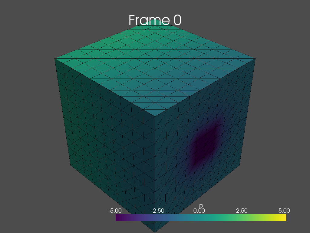
Fig. 4

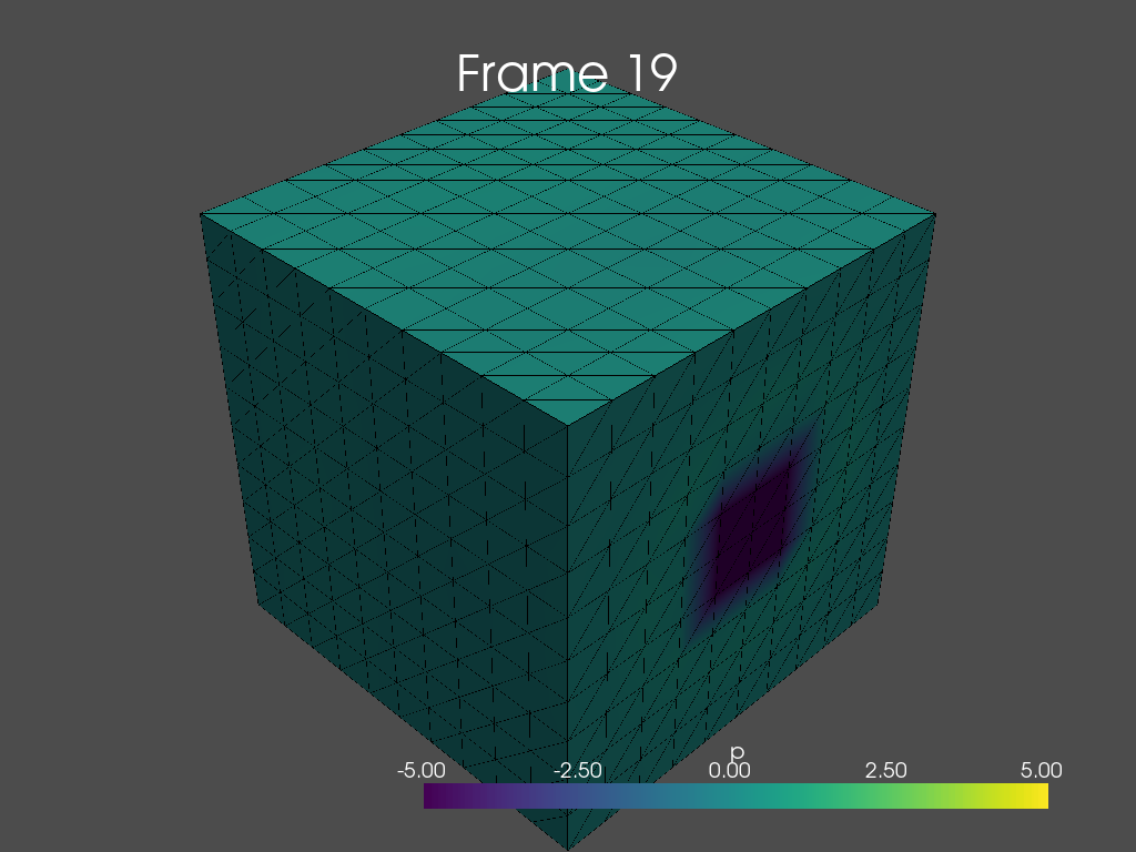
Fig. 5

Minimal code to reproduce (using Python 3.10.8 and fenics-dolfinx 0.5.2):

from mpi4py import MPI
from petsc4py import PETSc
import numpy as np
from scipy.spatial import distance
import pyvista

from dolfinx.fem import Constant, Function, FunctionSpace, assemble_scalar, dirichletbc, form, locate_dofs_topological
from dolfinx.fem.petsc import assemble_matrix, assemble_vector, apply_lifting, create_vector, set_bc
from dolfinx.mesh import locate_entities_boundary, create_unit_cube
from dolfinx.plot import create_vtk_mesh
from ufl import (FacetNormal, FiniteElement, Identity, TestFunction, TrialFunction, VectorElement,
                 div, dot, ds, dx, inner, lhs, nabla_grad, rhs, sym)
import os

mesh = create_unit_cube(MPI.COMM_WORLD, 10, 10, 10)

t = 0
T = 0.2
num_steps = 20
dt = T / num_steps

v_cg2 = VectorElement("CG", mesh.ufl_cell(), 2)
s_cg1 = FiniteElement("CG", mesh.ufl_cell(), 1)
V = FunctionSpace(mesh, v_cg2)
Q = FunctionSpace(mesh, s_cg1)

u = TrialFunction(V)
v = TestFunction(V)
p = TrialFunction(Q)
q = TestFunction(Q)


def inflow(x):
    accept_dist = 0.15
    return distance.cdist([[0, 0.5, 0.5]], x.T, 'euclidean') < accept_dist


def outflow(x):
    accept_dist = 0.15
    return distance.cdist([[1, 0.5, 0.5]], x.T, 'euclidean') < accept_dist


def boundary(x):
    return np.logical_not(np.logical_or(inflow(x), outflow(x)))


facetdim = mesh.topology.dim - 1
bndry_facets = locate_entities_boundary(mesh, facetdim, boundary)
wall_dofs = locate_dofs_topological(V, facetdim, bndry_facets)
u_noslip = np.array((0,) * mesh.topology.dim, dtype=PETSc.ScalarType)
bc_noslip = dirichletbc(u_noslip, wall_dofs, V)

inflow_facets = locate_entities_boundary(mesh, facetdim, inflow)
inflow_dofs = locate_dofs_topological(Q, facetdim, inflow_facets)
bc_inflow = dirichletbc(PETSc.ScalarType(5), inflow_dofs, Q)

outflow_facets = locate_entities_boundary(mesh, facetdim, outflow)
outflow_dofs = locate_dofs_topological(Q, facetdim, outflow_facets)
bc_outflow = dirichletbc(PETSc.ScalarType(-5), outflow_dofs, Q)
bcu = [bc_noslip]
bcp = [bc_inflow, bc_outflow]

u_n = Function(V)
u_n.name = "u_n"
U = 0.5 * (u_n + u)
n = FacetNormal(mesh)
f = Constant(mesh, PETSc.ScalarType((0, 0, 0)))  # CHANGED (0, 0) to (0, 0, 0) to adapt to 3D
k = Constant(mesh, PETSc.ScalarType(dt))
mu = Constant(mesh, PETSc.ScalarType(1))
rho = Constant(mesh, PETSc.ScalarType(1))


# Define strain-rate tensor
def epsilon(u):
    return sym(nabla_grad(u))


# Define stress tensor
def sigma(u, p):
    return 2 * mu * epsilon(u) - p * Identity(u.geometric_dimension())


# Define the variational problem for the first step
p_n = Function(Q)
p_n.name = "p_n"
F1 = rho * dot((u - u_n) / k, v) * dx
F1 += rho * dot(dot(u_n, nabla_grad(u_n)), v) * dx
F1 += inner(sigma(U, p_n), epsilon(v)) * dx
F1 += dot(p_n * n, v) * ds - dot(mu * nabla_grad(U) * n, v) * ds
F1 -= dot(f, v) * dx
a1 = form(lhs(F1))
L1 = form(rhs(F1))

A1 = assemble_matrix(a1, bcs=bcu)
A1.assemble()
b1 = create_vector(L1)

# Define variational problem for step 2
u_ = Function(V)
a2 = form(dot(nabla_grad(p), nabla_grad(q)) * dx)
L2 = form(dot(nabla_grad(p_n), nabla_grad(q)) * dx - (1 / k) * div(u_) * q * dx)
A2 = assemble_matrix(a2, bcs=bcp)
A2.assemble()
b2 = create_vector(L2)

# Define variational problem for step 3
p_ = Function(Q)
a3 = form(dot(u, v) * dx)
L3 = form(dot(u_, v) * dx - k * dot(nabla_grad(p_ - p_n), v) * dx)
A3 = assemble_matrix(a3)
A3.assemble()
b3 = create_vector(L3)

# Solver for step 1
solver1 = PETSc.KSP().create(mesh.comm)
solver1.setOperators(A1)
solver1.setType(PETSc.KSP.Type.BCGS)
pc1 = solver1.getPC()
pc1.setType(PETSc.PC.Type.HYPRE)
pc1.setHYPREType("boomeramg")

# Solver for step 2
solver2 = PETSc.KSP().create(mesh.comm)
solver2.setOperators(A2)
solver2.setType(PETSc.KSP.Type.BCGS)
pc2 = solver2.getPC()
pc2.setType(PETSc.PC.Type.HYPRE)
pc2.setHYPREType("boomeramg")

# Solver for step 3
solver3 = PETSc.KSP().create(mesh.comm)
solver3.setOperators(A3)
solver3.setType(PETSc.KSP.Type.CG)
pc3 = solver3.getPC()
pc3.setType(PETSc.PC.Type.SOR)


def u_exact(x):
    values = np.zeros((3, x.shape[1]), dtype=PETSc.ScalarType)  # CHANGED 2 to 3 to adapt to 3D
    values[0] = 4 * x[1] * (1.0 - x[1])
    return values


u_ex = Function(V)
u_ex.interpolate(u_exact)

L2_error = form(dot(u_ - u_ex, u_ - u_ex) * dx)

out_dir = 'velocity-3D'
p_out_dir = 'pressure-3D'
if not os.path.exists(out_dir):
    os.makedirs(out_dir)
if not os.path.exists(p_out_dir):
    os.makedirs(p_out_dir)

topology, cell_types, geometry = create_vtk_mesh(V)
# Create a point cloud of glyphs
function_grid = pyvista.UnstructuredGrid(topology, cell_types, geometry)

p_topology, p_cell_types, p_geometry = create_vtk_mesh(Q)
p_grid = pyvista.UnstructuredGrid(p_topology, p_cell_types, p_geometry)
# Create a pyvista-grid for the mesh
grid = pyvista.UnstructuredGrid(*create_vtk_mesh(mesh, mesh.topology.dim))

for i in range(num_steps):
    # Update current time step
    t += dt

    # Step 1: Tentative velocity step
    with b1.localForm() as loc_1:
        loc_1.set(0)
    assemble_vector(b1, L1)
    apply_lifting(b1, [a1], [bcu])
    b1.ghostUpdate(addv=PETSc.InsertMode.ADD_VALUES, mode=PETSc.ScatterMode.REVERSE)
    set_bc(b1, bcu)
    solver1.solve(b1, u_.vector)
    u_.x.scatter_forward()

    # Step 2: Pressure correction step
    with b2.localForm() as loc_2:
        loc_2.set(0)
    assemble_vector(b2, L2)
    apply_lifting(b2, [a2], [bcp])
    b2.ghostUpdate(addv=PETSc.InsertMode.ADD_VALUES, mode=PETSc.ScatterMode.REVERSE)
    set_bc(b2, bcp)
    solver2.solve(b2, p_.vector)
    p_.x.scatter_forward()

    # Step 3: Velocity correction step
    with b3.localForm() as loc_3:
        loc_3.set(0)
    assemble_vector(b3, L3)
    b3.ghostUpdate(addv=PETSc.InsertMode.ADD_VALUES, mode=PETSc.ScatterMode.REVERSE)
    solver3.solve(b3, u_.vector)
    u_.x.scatter_forward()
    # Update variable with solution form this time step
    u_n.x.array[:] = u_.x.array[:]
    p_n.x.array[:] = p_.x.array[:]

    # Write solutions to file
    # xdmf.write_function(u_n, t)
    # xdmf.write_function(p_n, t)

    # Create plotter
    plotter = pyvista.Plotter(off_screen=True)
    p_plotter = pyvista.Plotter(off_screen=True)
    p_plotter.add_title("Frame {}".format(i))
    p_plotter.add_mesh(grid, style="wireframe", color="k")
    p_grid["p"] = p_n.x.array.real
    p_plotter.add_mesh(p_grid, cmap='viridis')

    values = np.zeros((geometry.shape[0], 3), dtype=np.float64)
    values[:, :len(u_n)] = u_n.x.array.real.reshape((geometry.shape[0], len(u_n)))
    function_grid["u"] = values
    glyphs = function_grid.glyph(orient="u", scale=True, factor=1)

    plotter.add_title("Frame {}".format(i))
    plotter.add_mesh(grid, style="wireframe", color="k")
    plotter.add_mesh(glyphs, cmap='jet')
    plotter.view_vector([0.5, -0.5, 0.5])
    p_plotter.view_vector([0.5, -0.5, 0.5])
    plotter.screenshot("{}/{}_glyphs.png".format(out_dir, i))
    p_plotter.screenshot("{}/{}_pressure.png".format(p_out_dir, i))

    # Compute error at current time-step
    error_L2 = np.sqrt(mesh.comm.allreduce(assemble_scalar(L2_error), op=MPI.SUM))
    error_max = mesh.comm.allreduce(np.max(u_.vector.array - u_ex.vector.array), op=MPI.MAX)
    # Print error only every 20th step and at the last step
    if (i % 20 == 0) or (i == num_steps - 1):
        print(f"Time {t:.2f}, L2-error {error_L2:.2e}, Max error {error_max:.2e}")

[nate]

Your BCs are not consistent with the original problem. You have a discontinuity in the velocity between your no slip and inlet / outlet. So you’re likely seeing the Gibbs phenomenon in your quiver plot. Consider Couette flow - Wikipedia and particularly Hagen–Poiseuille equation - Wikipedia.

[georg]

@nate Many thanks for the quick reply! The Gibbs phenomenon as an explanation sounds reasonable. Does it imply that the CFD inside the mesh is correct and I only have to remove the velocity vectors outside the mesh? If not, would using Navier-Stokes equations instead of the Hagen-Poiseuille equation solve the issue since the latter is derived from the former? I have read that Couette flow is for CFD within two parallel plates, but I want to extend the above code to CFD inside custom meshs like blood vessels. So unfortunately, Couette flow is not general enough.
(PS: I am not a physicist or mathematician)

[nate]

I provided the two links to Couette and Poiseuille flow as examples of how you need to consider the physics of your problem in the imposition of boundary conditions; not as a replacement for your FE model.

I’m not sure off the top of my head what a consistent “far field” boundary condition for the inlet and outet flows would be for a rectangular hole. But perhaps you can work it out guided by the derivation of Couette and Poiseuille flow equations. If you had cylindrical holes it would trivially be a Poiseuille flow inlet and outlet.

Another approach is apply some parabolic inlet/outlet flow which may be “good enough”. Or add long thin channels to your inlet and outlet holes in your mesh so that any inconsistencies in the flow are allowed to develop to be physically relevant by the time they reach the holes in the main box volume.

[georg]

@nate I think your last suggestion fits best to my use case! How to know that those supporting pipes are long enough to make the inconsistencies in the flow negligible?

[nate]

I’m unfamiliar with any work on its analysis, so my avenue of investigation would be numerical experiments.