From the electric field between two conductors: the resulting total force

[Nexius]

Dear all.

I’m working on the 3D capacitor model: sphere in front of plane. I can solve the electrostatic potential with FEniCS, and I also obtain the 3D electrostatic field (well, I still have to improve this.)

In general, the overall force F in z-direction between the two conductors is given by:

F = 1/2 * eps_0 * int( E^2 * n_z *dS )

S is the conductor’s shapes and n_z is the z-component of the surface normal.

Question: can the force be calculated via FEniCS? It should be feasible, because the geometry of the conductors and the electrostatic field are already at hand … . Thanks for a small comment.

PS: So, the integral looks like this:

F is the force along the axis (z-direction). E is the electric field magnitude and n_z is the z component of the outward surface normal of St.

[Nexius]

Well, I look for something that is similar to GetDP, where the following is computed by the solver:

PostProcessing {
  { Name EleSta_v; NameOfFormulation Electrostatics_v;
    Quantity {
      ...
      { Name C;
        Value {
          Integral { [ 2.0*Pi*epsr[] * SquNorm[{Grad v}] ]; In DomainCC_Ele;
                      Integration GradGrad; Jacobian VolAxi; }
        }
      }
    }
  }
}

Does any equivalent post-processing exist also in FEniCS, any ideas?

[Nexius]

So, it is me who gives the correct answer, if true. - obviously, many thought that it is too trivial!

Everything stands here (well hidden). So one can obviously start with this ‘energy’ term:

energy = 0.5*dot(grad(u), grad(u))*dx

I will poste again if this is indeed doing the thing!

[bleyerj]

Hi,
in order to maximize your chances of obtaining an answer, you should first follow the guidelines, especially concerning posting a Minimal Working Example. Without that it is hard to help you without a code.
In any case, I would expect something like:

n = FacetNormal(mesh)
assemble(Constant(epsilon_0)/2*dot(grad(v), grad(v))*n[2]*ds(1))

assuming that your surface S_t has been tagged as 1 and if grad(v) is the electrostatic field.

[Nexius]

Dear bleyerj,

thanks for your answer, and sorry for the late reply.

@bleyerj

posting a Minimal Working Example

Yep, absolutely right, I should have done this. I got the same as you, despite this n = FacetNormal(mesh): I wasn’t that sure how to apply this … . Thanks.

So, here is the complete code. What I do is modelling the sphere-plane interaction.

import pygmsh
import meshio
from fenics import *

import matplotlib.pyplot as plt
import numpy as np
import scipy.constants as const
import os

# _____________________________________________________ The values to play with

# The potentials on the boundaries (inner and outer sphere)
pot_sphere = 10.0
pot_plane  =  0.0

# The position and size of the domain
domain_size      =  40.0
domain_x1        =  -domain_size/2.0
domain_y1        =  -domain_size/2.0
domain_z1        =  -domain_size/2.0
domain_x2        =   domain_size
domain_y2        =   domain_size
domain_z2        =   domain_size

# Offset used to move sphere + plane along z.
sphere_plane_z_offset = -domain_size / 4.0

# The position and size of the sphere
sphere_x =   0.0
sphere_y =   0.0
sphere_z =   3.5
sphere_r =   3.0
# sphere_z - sphere_r is the sphere-plane distance

# The position and size of the plane
plane_size      =  30.0
plane_height    =   1.0
plane_x1        =  -plane_size/2.0
plane_y1        =  -plane_size/2.0
plane_z1        =  -plane_height
plane_x2        =   plane_size
plane_y2        =   plane_size
plane_z2        =   plane_height

# The mesh precision
mesh_prec_domain  = 1.8
mesh_prec_ball    = 0.5
mesh_prec_plane   = 2.0

# ____________________________________________________________________ The code

text_spaces = "    "
dir_base = "./" + os.path.basename(__file__)[:-3]
if not os.path.isdir(dir_base):
    os.mkdir(dir_base)

# Build the mesh first with pygmsh
geom = pygmsh.opencascade.Geometry()

# Create the domain, sphere and plane, and ...
domain = geom.add_box([domain_x1, domain_y1, domain_z1],
                      [domain_x2, domain_y2, domain_z2],
                       char_length=mesh_prec_domain)

sphere = geom.add_ball([sphere_x,
                        sphere_y,
                        sphere_z+sphere_plane_z_offset],
                        sphere_r,
                        char_length=mesh_prec_ball)

plane   = geom.add_box([plane_x1, plane_y1, plane_z1+sphere_plane_z_offset],
                       [plane_x2, plane_y2, plane_z2],
                       char_length=mesh_prec_plane)


# ... take the difference (boolean).
space_1 = geom.boolean_difference([domain],[sphere],
                                   delete_first=True,
                                   delete_other=True)

space_2 = geom.boolean_difference([space_1],[plane],
                                   delete_first=True,
                                   delete_other=True)

# Sphere
geom.add_raw_code("Physical Surface(\"1\") = {20};")
# Plane below sphere
geom.add_raw_code("Physical Surface(\"2\") = {8,9,10,11,12,13};")
# Space
geom.add_raw_code("Physical Surface(\"3\") = {14,15,16,17,18,19};")
# Volume
geom.add_raw_code("Physical Volume(\"4\") = {" + space_2.id + "};")

# Build the .geo file.
mesh = pygmsh.generate_mesh(geom, geo_filename=os.path.join(dir_base,"structure.geo"))

# What follows is this mesh conversion stuff ... .
tetra_cells    = None
tetra_data     = None
triangle_cells = None
triangle_data  = None

for key in mesh.cell_data_dict["gmsh:physical"].keys():
    if key == "triangle":
        triangle_data = mesh.cell_data_dict["gmsh:physical"][key]
    elif key == "tetra":
        tetra_data = mesh.cell_data_dict["gmsh:physical"][key]

for cell in mesh.cells:
    if cell.type == "tetra":
        if tetra_cells is None:
            tetra_cells = cell.data
        else:
            tetra_cells = np.vstack([tetra_cells, cell.data])
    elif cell.type == "triangle":
        if triangle_cells is None:
            triangle_cells = cell.data
        else:
            triangle_cells = np.vstack([triangle_cells, cell.data])

tetra_mesh = meshio.Mesh(points=mesh.points,
                         cells={"tetra": tetra_cells},
                         cell_data={"name_to_read":[tetra_data]})

triangle_mesh =meshio.Mesh(points=mesh.points,
                           cells=[("triangle", triangle_cells)],
                           cell_data={"name_to_read":[triangle_data]})
meshio.write(os.path.join(dir_base,"tetra_mesh.xdmf"), tetra_mesh)
meshio.write(os.path.join(dir_base,"mf.xdmf")        , triangle_mesh)

# All the latter .xdmf files are read such that they can be used in FEniCS.
mesh = Mesh()
with XDMFFile(os.path.join(dir_base,"tetra_mesh.xdmf")) as infile:
    infile.read(mesh)

mvc = MeshValueCollection("size_t", mesh, 2)
with XDMFFile(os.path.join(dir_base,"mf.xdmf")) as infile:
    infile.read(mvc, "name_to_read")
mf = cpp.mesh.MeshFunctionSizet(mesh, mvc)

mvc2 = MeshValueCollection("size_t", mesh, 3)
with XDMFFile(os.path.join(dir_base,"tetra_mesh.xdmf")) as infile:
    infile.read(mvc2, "name_to_read")
cf = cpp.mesh.MeshFunctionSizet(mesh, mvc2)


dx = Measure("dx", domain=mesh, subdomain_data=cf)
ds = Measure("ds", domain=mesh, subdomain_data=mf)

V = FunctionSpace(mesh, 'P', 2)

boundary_sphere  = DirichletBC(V, Constant(pot_sphere), mf, 1)
boundary_plane   = DirichletBC(V, Constant(pot_plane),  mf, 2)

# This is the boundary at the 5 sides of the domain cube. We say here that
# the potential at the boundary is the one of the sphere being with,
# e.g., 10V * r_sphere / r.
pot_b = Expression('(pot*rs) / sqrt(pow(x[0]-rx, 2) + pow(x[1]-ry, 2) + pow(x[2]-rz, 2))',
                   degree=1, rx=sphere_x, ry=sphere_y, rz=sphere_z,
                   pot=pot_sphere, rs=sphere_r)

# Otherwise, we could simply put the potential at the 5 sides onto 0, which I
# would personallt find strange.
#pot_b = Constant(0.0)

boundary_space  = DirichletBC(V, pot_b, mf, 3)
bcs =[boundary_sphere, boundary_plane, boundary_space]

u = TrialFunction(V)
v = TestFunction(V)
a = dot(grad(u), grad(v)) * dx
L = Constant('0') * v * dx
u = Function(V)
solve(a == L, u, bcs)

electric_field = project(-grad(u))

potentialFile = File(os.path.join(dir_base,"Potential.pvd"))
potentialFile << u
e_fieldfile   = File(os.path.join(dir_base,"Efield.pvd"))
e_fieldfile   << electric_field

# Now comes the force, calculated from the potential.
# ds(1) -> boundary No. 1 -> the sphere (see above)
# n[2]  -> z-component of the normal vector
# The force is in nN.
n  = FacetNormal(mesh)
force_n = assemble(  dot(grad(u), grad(u))*n[2]*ds(1)  )
force_n = force_n * (const.epsilon_0/2.0)
print("")
print("")
print(text_spaces + "Force,  numerical: " + str(force_n))

# Here is the analytical result for the force. The equation was taken from
# S. Hudlet, M. Saint Jean, C. Guthmann, J. Berger, Eur. Phys. J. B 2, 5 (1998)
# F = Pi * eps_0 * ( R^2/(z*(z+R)) ) * V^2
# Note that the plane is infinitesimal large
dist_z = sphere_z-sphere_r
dist_f = sphere_r**2.0 / (dist_z * (dist_z+sphere_r))
force_a  = const.pi * const.epsilon_0 * dist_f * (pot_plane - pot_sphere)**2.0
print(text_spaces + "Force, analytical: " + str(force_a))
print("")
print("")

f= open(os.path.join(dir_base,"Forces.txt"),"w+")
f.write("Force,  numerical: " + str(force_n) + "\n"
        "Force, analytical: " + str(force_a))
f.close()

Things seem to work because I obtain almost the same force value (in nN) as I would obtain with the analytic formula:

Force,  numerical: 1.2271093819360867e-08
Force, analytical: 1.4305500720689379e-08

However, there are some questions I would like to ask if you do not mind:

Q1: Although surprisingly quite close, the numerical force values are always smaller than the corresponding ‘analytic’ values, independent on the parameters (sphere size, distance, mesh size, etc.). Is this normal? Could it be that my mesh is not sufficiently precise enough or that the plane is not infinitesimal large enough? Or is there even a mistake in my code?

Q2: The mesh resolution above is almost the max I can have. Otherwise, I get an ‘out of memory’ error:

UMFPACK V5.7.1 (Oct 10, 2014): ERROR: out of memory

Is there a way to circumvent this? I use FEniCS in a docker environment (latest version) on a standad laptop computer.

Q3: It would be nice if you could give me some help/ideas/feelings/etc here at this point: what concerns the boundary of the domain, one can put the sides of the cube onto 0V (see first image). But one can also assume the potential of only the sphere (voltage of sphere x radius of sphere / distance), see image No.2. Is there some rule of thumb what has to be done in electrostatics for ‘open’ boundaries? This 1/r dependence is somewhat mentioned in one book and one publication without any details.

Thanks for some feedback.

[bilenemek]

Dear Nexius

The best assumption is “far away” condition meaning that far away from the object the electric field and magnetic flux vanish. Since the electromagnetic potentials (in your case, only the electric potential, \phi) is the solution of the electric field

E_i =- \phi_{,i}

setting \phi=0 at the computational boundaries would be adequate. By doing 2-3 times the radius far from the edges of the rectangle would be a good attempt for this boundary condition. The rule of thumb is really this, nothing more. If you want to find out accurately the smallest distance, a convergence study would help: three geometries close, far, very far away boundaries, evaluating the electric field at the same position, calculating an error.

For such computations, I can also suggest to have a look at the Chapter 3.2 Polarized Materials in the book Computational Reality, 2017, Springer. If your library does not give access to you, contact me per e-mail: http://bilenemek.abali.org

Best, Emek

[Nexius]

Dear bilenemek.

Thanks a lot for your interest and help!

@bilenemek

If you want to find out accurately the smallest distance, a convergence study would help: three geometries close, far, very far away boundaries, evaluating the electric field at the same position, calculating an error.

This is what I have done the last days. I modified the code from above such that I obtain a force versus distance curve (see Figure 1) where I then compare the analytical with the FEM result (I also calculate the error, see Figure 2). I varied many parameters and what comes out can be concluded as follows:

1. Conclusion - values
Almost ‘independent’ on the sphere size, mesh ‘quality’, even the plane size and the domain size, I always have a large error of about 15 to 20% for close distances (z < r_sphere) and one at large distances (z > r_sphere). Roughly around a distance comparable to the sphere’s size, a minimum is obtained, see Figure 2. Of course, if the mesh has a bad quality (in particular at the sphere and below, on the plane) the error values start to raise. There is also some improvement when the domain is increased. Unfortunately, I cannot go to very fine meshes because my laptop is out of memory then (UMFPACK V5.7.1 (Oct 10, 2014): ERROR: out of memory).

2. Conclusion - boundary model
I used three boundary models: 1) the potential is zero at all the boundaries, 2) the potential is V_sphere * r_sphere / r at all boundaries and 3) the same as a) despite the face below the plate which is put onto zero. Note that the plate is also on zero potential.
As it can be seen in the figure, the 1/r boundary condition is better (Model 2 and 3) than the zero boundary condition (Model 1). This is somehow in agreement with the few literature [1-3] I was reading meanwhile: basically a 1/r ‘correction’ accounts for the ‘rest’ field at these places. A Robin condition should be used [3] which I have not yet introduced.

[1] The Finite Element Method in Electromagnetics, Jin, Jianming, page 184
[2] A. J. Otto, N. Marais, E. Lezar, and D. B. Davidson, IEEE Antennas Propag. Mag. 54, 206 (2012). page 209
[3] [1] O. A. Basaran and L. E. Scriven, Phys. Fluids A Fluid Dyn. 1, 795 (1989).

So, after all I’m somewhat happy but I’m concerned about the relatively large errors of ~20% and more.

Question 1: are these deviations normal in FEM?

Question 2: might it be that in order to improve the result I need a super computer to refine much the mesh so that the entire thing well converges? So the dream to use a simple laptop for research simulations is simply a stupid idea?

Question 3: could it be that there is a mistake in my code?

Thanks for some comments … .

[Nexius]

Dear all.

So, I played around with the model and found my personal best ‘convincing’ solution … so far. A full example is shown here, which is a minimal MWE of the current code:

import matplotlib.pyplot as plt
import numpy as np
import scipy.constants as const
import os

# _____________________________________________________ The values to play with

# Main parameters
pot_sphere         =    3.0 # Potential of the sphere
pot_plane          =    0.0 # Potential of the plane
sphere_r           =    3.0 # Radius of the sphere
domain_size        =   80.0 # Domain size (sphere)
plane_size         =   70.0 # Plane size
plane_height       =    0.5
scene_z_off        =  -16.0 # Z offset value for the sphere and plane
z                  =    1.0 # Distance sphere-plane (in nm)

mesh_prec_domain   =    6.0 # Precision of the mesh in the domain

# I use a bounding mesh box with a refined mesh around the sphere
mesh_prec_ball     =    0.3 # Mesh precision
# mesh_box_sl: lateral size in %, 1.0 = lateral size of the plane
# mesh_box_sh: height in %,
#     first value : towrads the plane,  1.0 = full height
#     second value: towrads the sphere, 1.0 = complete sphere is included
mesh_box_sl        =    0.15
mesh_box_sh        =    (1.0, 1.0)

# Other things
sphere_x           =    0.0
sphere_y           =    0.0
sphere_z           =    0.0
plane_x            =    0.0
plane_y            =    0.0
plane_z            =    0.0
plane_vx           =    0.0
plane_vy           =    0.0
plane_vz           =    0.0

# ___________________________________________________________________ Directory

text_spaces = "    "
dir_base = "./" + os.path.basename(__file__)[:-3]
if not os.path.isdir(dir_base):
    os.mkdir(dir_base)

# ____________________________________________________ Mesh creation via pygmsh

sphere_z   =  sphere_r + z

# The position and size of the plane
plane_z   = -plane_height
plane_vz  =  plane_height

# Build the mesh first with pygmsh
geom = pygmsh.opencascade.Geometry()

# Create the domain, sphere and plane, and ...

# The domain is a large sphere.
domain = geom.add_ball([0.0, 0.0, 0.0],
                        domain_size)

sphere = geom.add_ball([sphere_x,
                        sphere_y,
                        sphere_z+scene_z_off],
                        sphere_r)

plane   = geom.add_cylinder([plane_x,
                                plane_y,
                                plane_z+scene_z_off],
                            [plane_vx,
                                plane_vy,
                                plane_vz],
                            plane_size,
                            2.0*const.pi)

# ... take the difference (boolean).
space_1 = geom.boolean_difference([domain],[sphere],
                                    delete_first=True,
                                    delete_other=True)

space_2 = geom.boolean_difference([space_1],[plane],
                                    delete_first=True,
                                    delete_other=True)

# Sphere
geom.add_raw_code("Physical Surface(\"1\") = {7};")
# Plane below sphere
geom.add_raw_code("Physical Surface(\"2\") = {3,4,5};")
# Domain
geom.add_raw_code("Physical Surface(\"3\") = {6};")
# Volume
geom.add_raw_code("Physical Volume(\"4\") = {" + space_2.id + "};")

# The refined mesh in a bounding box around the sphere and the plane.
center_z = scene_z_off + z/2.0
z_min = center_z - z/2.0 - mesh_box_sh[0] * plane_height
z_max = center_z + z/2.0 + mesh_box_sh[1] * 2.0 * sphere_r
x_max =  (mesh_box_sl * plane_size) / 2.0
x_min = -(mesh_box_sl * plane_size) / 2.0
y_max = x_max
y_min = x_min

# We hard-code the refined mesh into the .geo file via the Field option.
geom.add_raw_code("//+")
geom.add_raw_code("Field[1] = Box;")
geom.add_raw_code("//+")
geom.add_raw_code("Field[1].VIn = "  + str(mesh_prec_ball)   + ";")
geom.add_raw_code("//+")
geom.add_raw_code("Field[1].VOut = " + str(mesh_prec_domain) + ";")
geom.add_raw_code("//+")
geom.add_raw_code("Field[1].XMax = " + str(x_max) + ";")
geom.add_raw_code("//+")
geom.add_raw_code("Field[1].XMin = " + str(x_min) + ";")
geom.add_raw_code("//+")
geom.add_raw_code("Field[1].YMax = " + str(y_max) + ";")
geom.add_raw_code("//+")
geom.add_raw_code("Field[1].YMin = " + str(y_min) + ";")
geom.add_raw_code("//+")
geom.add_raw_code("Field[1].ZMax = " + str(z_max) + ";")
geom.add_raw_code("//+")
geom.add_raw_code("Field[1].ZMin = " + str(z_min) + ";")
geom.add_raw_code("//+")
geom.add_raw_code("Background Field = 1;")

file_geo = os.path.join(dir_base, "Geometry.geo")
mesh = pygmsh.generate_mesh(geom, geo_filename=file_geo)

# ______________________________________________ Mesh conversion and re-reading

# What follows is this mesh conversion stuff ... .
tetra_cells    = None
tetra_data     = None
triangle_cells = None
triangle_data  = None

for key in mesh.cell_data_dict["gmsh:physical"].keys():
    if key == "triangle":
        triangle_data = mesh.cell_data_dict["gmsh:physical"][key]
    elif key == "tetra":
        tetra_data = mesh.cell_data_dict["gmsh:physical"][key]

for cell in mesh.cells:
    if cell.type == "tetra":
        if tetra_cells is None:
            tetra_cells = cell.data
        else:
            tetra_cells = np.vstack([tetra_cells, cell.data])
    elif cell.type == "triangle":
        if triangle_cells is None:
            triangle_cells = cell.data
        else:
            triangle_cells = np.vstack([triangle_cells, cell.data])

tetra_mesh = meshio.Mesh(points=mesh.points,
                         cells={"tetra": tetra_cells},
                         cell_data={"name_to_read":[tetra_data]})

triangle_mesh =meshio.Mesh(points=mesh.points,
                           cells=[("triangle", triangle_cells)],
                           cell_data={"name_to_read":[triangle_data]})
meshio.write(os.path.join(dir_base,"tetra_mesh.xdmf"), tetra_mesh)
meshio.write(os.path.join(dir_base,"mf.xdmf")        , triangle_mesh)

# All the latter .xdmf files are read such that they can be used in FEniCS.
mesh = Mesh()
with XDMFFile(os.path.join(dir_base,"tetra_mesh.xdmf")) as infile:
    infile.read(mesh)

mvc = MeshValueCollection("size_t", mesh, 2)
with XDMFFile(os.path.join(dir_base,"mf.xdmf")) as infile:
    infile.read(mvc, "name_to_read")
boundaries = cpp.mesh.MeshFunctionSizet(mesh, mvc)

mvc2 = MeshValueCollection("size_t", mesh, 3)
with XDMFFile(os.path.join(dir_base,"tetra_mesh.xdmf")) as infile:
    infile.read(mvc2, "name_to_read")
subdomains = cpp.mesh.MeshFunctionSizet(mesh, mvc2)

# ______________________________________ (Sub)domains, boundary conditions, etc.

dx = Measure("dx", domain=mesh, subdomain_data=subdomains)
ds = Measure("ds", domain=mesh, subdomain_data=boundaries)

# The mesh function.
V0 = FunctionSpace(mesh, "DG", 0)
V  = FunctionSpace(mesh, "P",  2)
#V  = FunctionSpace(mesh, "P",  2)

b_cond = []
#b_cond.append(DirichletBC(V, Constant(0.0), boundaries, 3)) # Main domain (large sphere)
b_cond.append(DirichletBC(V, Constant(pot_sphere), boundaries, 1)) # 1: sphere
b_cond.append(DirichletBC(V, Constant(pot_plane),  boundaries, 2)) # 2: plane

# Domain boundary (large sphere): Robin condition
# From: Basaran, Scriven, Phys. Fluids A Fluid Dyn. 1, 795 (1989).
#r = Constant(2.0)
r = Expression("sqrt(" \
            "pow(x[0]-rx, 2) + " \
            "pow(x[1]-ry, 2) + " \
            "pow(x[2]-rz, 2))", degree=1,
            rx=sphere_x, ry=sphere_y, rz=sphere_z)
p = 1 / r
q = Constant(0.0)

# Poisson equation with the source set to 0
u = TrialFunction(V)
v = TestFunction(V)
a = dot(grad(u), grad(v)) * dx + p * u * v * ds(3)
L = Constant('0') * v * dx + p * q * v * ds(3)

u = Function(V)
solve(a == L, u, b_cond, solver_parameters = {"linear_solver": "gmres",
                                              "preconditioner": "ilu"})
electric_field = project(-grad(u))

potentialFile = File(os.path.join(dir_base,"Potential.pvd"))
potentialFile << u
e_fieldfile   = File(os.path.join(dir_base,"Efield.pvd"))
e_fieldfile   << electric_field

# Force (in nN), calculated from the potential.
# ds(1) -> boundary No. 1 -> the sphere (see above)
# n[2]  -> z-component of the normal vector
n  = FacetNormal(mesh)
force_n = assemble(  dot(grad(u), grad(u))*n[2]*ds(1)  )
force_n = force_n * (const.epsilon_0/2.0)
print("\n\n" + text_spaces + "Force,  numerical: " + str(force_n))

# Here is the analytical result for the force. The equation was taken from
# S. Hudlet, M. Saint Jean, C. Guthmann, J. Berger, Eur. Phys. J. B 2, 5 (1998)
# F = Pi * eps_0 * ( R^2/(z*(z+R)) ) * V^2
dist_z = sphere_z-sphere_r
dist_f = sphere_r**2.0 / (dist_z * (dist_z+sphere_r))
force_a  = const.pi * const.epsilon_0 * dist_f * (pot_plane - pot_sphere)**2.0
print(text_spaces + "Force, analytical: " + str(force_a) + "\n")
print(text_spaces + "Error  (Fa-Fn)/Fa: " + str((force_a-force_n)/force_a*100.0) + " %\n")

I’m not really a 100% sure if I have done correctly the coding, also in an ‘intelligent way’, may be you have a look. With respect to the previous code from above, I changed the following things:

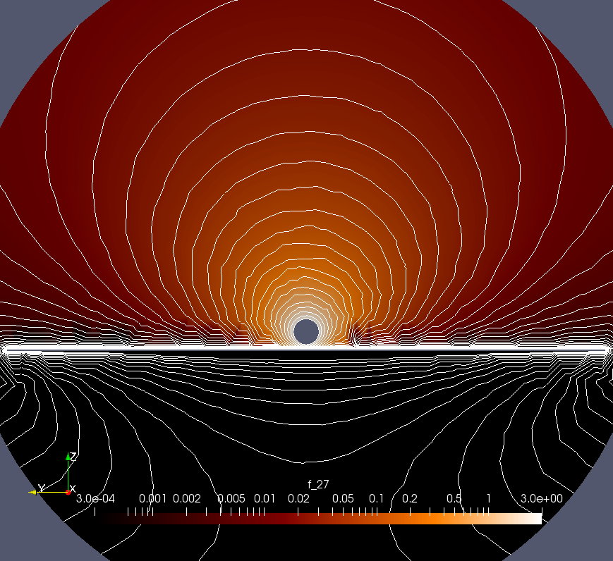
• I have chosen a spherical geometry: the domain is now a large sphere, and also the plane is a circular disk (thin cylinder) now (see image 1). This creates much better well-formed equipotential lines (see image 2, logarithmic color scale and scale for the lines!)

• The mesh of the region around the sphere and the plane underneath is now represented in a much finer mesh. This improves much the force value because most of the sphere-plane interaction is created there (see image 3). In fact, I hard-code via geom.add_raw_code a box with properties mesh_box_sl (lateral size) and mesh_box_sh (height) into the .geo file with the help of Field[1] = Box; etc. In my code, the mesh’s precision is is given by mesh_prec_ball whereas mesh_prec_domain is the precision of the mesh in the rest of the domain.

• I now use gmres as a linear solver and ilu as a pre-conditioner. With them, I can make use of fine meshes without ‘OUT OF MEMORY’ issues. Other linear solvers do not really improve the ‘OUT OF MEMORY’ issue but I’m still working on this.

• I apply a Robin boundary condition on the domain boundary (large sphere) with dphi/dr = phi/r, as described in Basaran, Scriven, Phys. Fluids A Fluid Dyn. 1, 795 (1989).

All these changes produce a much smaller error which is now around 8% with respect to the expected analytical force value, in the distance range of interest (between 0.5 and 3 nm).

Force,  numerical: 5.189529363356381e-10
Force, analytical: 5.632790908771443e-10
Error  (Fa-Fn)/Fa: 7.869305866205872 %

Questions

Q1: Does the mesh, which I’m using, make sense? I have the following statistics:

  Input points: 8521
  Input facets: 17030
  Input segments: 25545
  Input holes: 0
  Input regions: 0
  Mesh points: 8521
  Mesh tetrahedra: 41081
  Mesh faces: 85247
  Mesh edges: 52686
  Mesh faces on facets: 17030
  Mesh edges on segments: 25545

Is the mesh size still too large?
When decreasing the mesh size in the domain, not much changes. It is only in the region around the sphere that is quite sensitive to the mesh size, which makes sense because most of the sphere-plane interaction is created there … . To my opinion, one has to increase even more the mesh. What do you think?

Q2: The latter brings me to the limits of my laptop. With the parameters from above I’m at the full limit: if I lower the mesh size a bit I obtain an ‘OUT OF MEMORY’.
Is it possible to calculate only, e.g., a quarter of the sphere-plane structure since the electrostatic field and potential is highly symmetric around the z-axis?
Other (bad) idea: if I model the sphere-plane in 2D, I will not obtain the right force, right? In other words, a 3D case needs to be modeled in 3D in FEM, is this right?

Q3: I would like to play with the parameters of the solver and have read the manual Solving PDEs in Python – The FEniCS Tutorial Volume I (page 119). How can I change the following code

u = Function(V) 
problem = LinearVariationalProblem(a, L, u, bc) 
solver = LinearVariationalSolver(problem) 
solver.parameters.linear_solver = ’gmres’ 
solver.parameters.preconditioner = ’ilu’ 
prm = solver.parameters.krylov_solver # short form 
prm.absolute_tolerance = 1E-7 
prm.relative_tolerance = 1E-4 
prm.maximum_iterations = 1000
solver.solve()

such that it works? I obtain an error at prm = solver.parameters.krylov_solver

Because I’m still quite new to FEM applications I still need some help. Any help is highly appreciated. Thanks in advance.

[J_1]

Preface: I have little experience with Fenics. I have been following this forum in hopes of learning. Most of my simulation experience has been with commercial fem solvers for high frequency electromagnetics, but some simulation strategies I’ve learned should apply to electrostatics too.

1). When available memory is limited, use an iterative solver such as gmres. Direct solvers such as umfpack are much faster, but as you’ve seen require much more memory.
2). Always try to exploit problem symmetry to reduce memory requirements. Your specific problem has two symmetry planes and the D.O.F. can be reduced by a factor of 4.
See this blog series for an example of exploiting symmetry. When you reduce your simulation domain by exploiting symmetries, you will have to account for this reduction when calculating quantities involving integration over a spatial dimension.
3). Meshes should be the most dense where the unknown for which you are solving changes rapidly.
4). Even on fast computers, solving a 3D problem can take a long time. I always try to start with a similar 2D problem. In 2D, I would test my weak formulation, explore boundary conditions including symmetry boundary conditions to reduce problem size, perform a convergence study to determine the minimum possible size of my simulation domain, perform a convergence study for mesh element size, etc. Although there is no 2D equivalent of your problem, a similar 2D problem would be that of a wire over an infinite ground plane (for which an analytical solution exists).

Speaking of analytical solutions, the equation you cited in your code assumes an infinite ground plane. The results you’ve shared have a finite ground plane, which may be a cause for the discrepancy you’ve observed between the analytical solution and numerical simulation.

As you’ve shown in your presented results, the electric field is near zero beneath the ground plane. Thus, you shouldn’t need to simulate the region beneath the ground plane. To further reduce the computational requirements, I would try placing the ground plane at the very bottom of your simulation domain and extend the ground plane until the edge of your simulation domain where you are applying the Robin condition.

Hope this helps. I look forward to seeing your results when you’ve figured out everything.

[bilenemek]

Dear Nexius

Good to see that you found the iterative solver for larger problems, especially in electromagnetism, the choice of the iterative solver is an issue, I would suggest to go a pragmatic way and use different ones (with and without preconditioners). Please use another units or increase the tolerance, as your force value is smaller than the error tolerance, which might be an issue when you compare results.

Your pde is linear, but you can always use the nonlinear solution method, so it converges in one Newton–Raphson iteration, as follows:

u = Function(V)
du = TrialFunction(V)
v = TestFunction(V)
a = dot(grad(u), grad(v)) * dx + p * u * v * ds(3)
L = Constant(‘0’) * v * dx + p * q * v * ds(3)

Form = a - L
Gain = derivative(Form,u,du)

problem = NonlinearVariationalProblem(Form, u, b_cond, Gain)
solver = NonlinearVariationalSolver(problem)

solver.parameters[“newton_solver”][“relative_tolerance”] = 1E-9
solver.parameters[“newton_solver”][“absolute_tolerance”] = 1E-10
solver.parameters[“newton_solver”][“convergence_criterion”] = “residual”
solver.parameters[“newton_solver”][“error_on_nonconvergence”] = True
solver.parameters[“newton_solver”][“linear_solver”] = “gmres”
solver.parameters[“newton_solver”][“lu_solver”][“symmetric”] = True
solver.parameters[“newton_solver”][“maximum_iterations”] = 100
solver.parameters[“newton_solver”][“preconditioner”] = “amg”
solver.parameters[“newton_solver”][“relaxation_parameter”] = 1.05
solver.parameters[“newton_solver”][“report”] = False

solver.parameters[“newton_solver”][“krylov_solver”][“nonzero_initial_guess”] = True
solver.parameters[“newton_solver”][“krylov_solver”][“relative_tolerance”] = 1E-5
solver.parameters[“newton_solver”][“krylov_solver”][“absolute_tolerance”] = 1E-7
solver.parameters[“newton_solver”][“krylov_solver”][“monitor_convergence”] = False
solver.parameters[“newton_solver”][“krylov_solver”][“maximum_iterations”] = 100000

solver.solve()

Furthermore, I had a look at the paper, where you found the analytic result. It is difficult to judge for me since I do not know the image method that they are referring to. Also the number of used expansion is not given, so consider the case that their approximative solution method includes also a few per cent errors.

One important note is on your choice of quadratic elements. As the electric potential is solved within the finite element with a degree 2 shape function, electric field will be linear within the element; but across elements, electric field is still discontinuous—technically not so bad, since you apply E_i n_i=0 between internal boundaries at integrating by part, not on purpose, but you do that helps a lot; another issue might be the surface charge \varepsilon_0 E_i n_i=\sigma in the paper on the electrode surface. There is no real benefit for your application to use quadratic elements, simply use linear and even a finer mesh between the disc and electrode tip.

Best, Emek

[Nexius]

Dear bilenemek.

Thanks a lot for your propositions, this really helped a lot! And sorry for being so late - during the last days, I have worked on my more complicated models and have read also some literature about electrostatics and FEM. BTW, a good introduction into FEniCS for beginners like me is this lecture course.

Here some comments:

@bilenemek

Please use another units or increase the tolerance, as your force value is smaller than the error tolerance, which might be an issue when you compare results.

The point is that in the force calculation …

n  = FacetNormal(mesh)
force_n = assemble(  dot(grad(u), grad(u))*n[2]*ds(1)  )
force_n = force_n * (const.epsilon_0/2.0)

the small values are due to epsilon_0, which is, however, multiplied after the assemble call. So, things should be okay.

@bilenemek

Your pde is linear, but you can always use the nonlinear solution method, so it converges in one Newton–Raphson iteration, as follows:

Thank you so much, this really helps! All this is included now. What I found out is that the following values …

solver.parameters[“newton_solver”][“relative_tolerance”] = 1E-2
solver.parameters[“newton_solver”][“absolute_tolerance”] = 1E-3

… are sufficient to obtain a ‘first good guess’. I also realized that this …

electric_field = project(-grad(u))

also takes some long calculation time. It is now (de-)activated by a switch because I don’t always need it.

@bilenemek

Furthermore, I had a look at the paper, where you found the analytic result. It is difficult to judge for me since I do not know the image method that they are referring to. Also the number of used expansion is not given, so consider the case that their approximative solution method includes also a few per cent errors.

What the people have found is that the solution is actually a very good one, if you consider the solution for the capacitance …

… to be the ‘exact and true’ one (Note: Force = 1/2 * diff(C,z) V², and λ = (R + z)/R). If you are interested, I can send some papers … .

@bilenemek

There is no real benefit for your application to use quadratic elements, simply use linear and even a finer mesh between the disc and electrode tip.

Yep okay, thanks for the hint.

[bilenemek]

Because you mentioned that the project takes a long time, you can fine tune it by choosing the solver and number of Gauss points more wisely:

project(-grad(u), VectorFunctionSpace(mesh,‘P’,1), solver_type=“mumps”, form_compiler_parameters={“cpp_optimize”: True, “representation”: “uflacs”, “quadrature_degree”: 2} )

Best, Emek

[Nexius]

Dear bilenemek,

cool, thanks a lot! Q1: Is this way of calculation more accurate than what I have used before?

project(-grad(u))

I have two other questions:

Q2: At the moment, I simulate a 2nd metallic sphere that is in between the first sphere and the plane from above (the latter both are still on their well-defined Dirichlet potentials, as above). This new second sphere has no Dirichlet defined potential, and what I want to see is the induction created by the E-field between the first sphere and plane. So, although the total charge is zero on the 2nd sphere, there is charge separation, similar to this:

How can I simulate electrostatic induction in FEniCS? What I have done is to assign a new sub-domain for the second sphere. There, I define a new epsilon, which I basically put onto a very high value (e.g., 1.0e15) such that I simulate a ‘metal’. So far, it looks good. But I ask myself if it is really the way to go. What do you think?

Q3: On the latter 2nd sphere, we have a charge redistribution. With …

… I can calculate the surface charge density roh on the sphere. Of course, I can calculate this in FEniCS (I still don’t know how …), however, how can I show this in Paraview on the sphere?

Thanks in advance for some ideas … .

[bilenemek]

Q1: No, it is not more or less accurate, but you have a control on the solver. If the number of degrees of freedom is more than 100k, your computer may have difficulties since the RAM consumption will be too high. In this case using an iterative method might be handy.

Q2: Equations are the same, you may like to have a look at my book (see previous answer of mine). If you want to visualize charge per mass, z, simply use the Maxwell equation for that \rho z = D_{i,i} with the charge potential D_i=\epsilon E_i. By the way metals are conductive, you should use conductivity not the permittivity.

Q3: Surface charge is then simply q=n_i [D_i] with jump brackets [D_i]=D_i^+-D_i^- being plus and minus on both sides of the singular surface between two materials. Project this and try to visualize in Paraview, since charge potential is continuous, within same material domains, it will vanish.

[Nexius]

Hi bilenemek,

thanks again for your help! At the end of this message you find a MWE of what I have described above. Here are some comments:

@bilenemek

Q1: No, it is not more or less accurate, but you have a control on the solver.

Okay, I see, thx.

@bilenemek

you may like to have a look at my book (see previous answer of mine)

I would really like to, however, my university has no access so far. I need to see.

@bilenemek

By the way metals are conductive, you should use conductivity not the permittivity.

Sure they are (!) , but I was asking myself how to implement this into FEniCS in terms of field induction. The reason is that you cannot impose a boundary condition for sphere No2. At the end I had then the idea to increase the eps of a ‘dielectric sphere’ towards infinity such that it gets ‘metallic’.

@bilenemek

Surface charge is then simply q=ni[Di]q=n_i [D_i] with jump brackets [Di]=D+i−D−i[D_i]=D_i^±D_i^- being plus and minus on both sides of the singular surface between two materials.

Hmmm, I think I need your chapter. Is that coded as you have written?

MWE
Here is the capacitor arrangement:

The yellow sphere is on potential 0V and the plane on +10V. The greenish sphere has no Dirichlet defined potential and is charge neutral. It forms a sub-domain with an eps, which I have put onto a very high value of 10⁶. Here is the code:

import pygmsh
import meshio
from fenics import *

import matplotlib.pyplot as plt
import numpy as np
import scipy.constants as const
import os

# _____________________________________________________ The values to play with

# Main parameters
pot_sphere         =    0.0 # Potential of the sphere
pot_plane          =   10.0 # Potential of the plane
sphere_r           =    8.0 # Radius of the sphere
sphere2_r          =    6.0 # Radius of the 2nd sphere
z                  =    5.0 # Distance sphere-sphere2 (in nm)
z2                 =    5.0 # Distance sphere2-plane  (in nm)

domain_size        =   80.0 # Domain size (sphere)
plane_size         =   70.0 # Plane size
scene_z_off        =  -16.0 # Z offset value for the sphere and plane

eps_sphere2        =    1.0e6 # a high eps value for a metal
eps_domain         =    1.0

mesh_prec_domain   =    8.0 # Precision of the mesh in the domain
# I use a bounding mesh box with a refined mesh around the sphere
mesh_prec_ball     =    0.8 # Mesh precision in the box
# mesh_box_sl: lateral size in %, 1.0 = lateral size of the plane
# mesh_box_sh: height in %,
#     first value : towrads the plane,  1.0 = full height, including sphere2
#     second value: towrads the sphere, 1.0 = complete sphere is included
mesh_box_sl        =    0.30
mesh_box_sh        =    (1.0, 1.0)

# Other things
sphere_x           =    0.0
sphere_y           =    0.0
sphere2_x          =    0.0
sphere2_y          =    0.0
plane_x            =    0.0
plane_y            =    0.0
plane_vx           =    0.0
plane_vy           =    0.0

# ___________________________________________________________________ Directory

text_spaces = "    "
dir_base = "./" + os.path.basename(__file__)[:-3]
if not os.path.isdir(dir_base):
    os.mkdir(dir_base)

# ____________________________________________________ Mesh creation via pygmsh

geom = pygmsh.opencascade.Geometry()

# The domain is a large sphere.
domain = geom.add_ball([0.0, 0.0, 0.0],
                        domain_size)

# The sphere, which is on a potential
sphere_z  = sphere_r + z
sphere    = geom.add_ball([sphere_x, sphere_y, sphere_z+scene_z_off], sphere_r)

# The second sphere, where we want to observe induction
sphere2_z = -sphere2_r
sphere2   = geom.add_ball([sphere2_x, sphere2_y, sphere2_z+scene_z_off],
                          sphere2_r)

# The plane, which cuts the large spherical domain, also on a defined potential.
plane_z   = -domain_size * 1.5 -z2 - 2.0 * sphere2_r - 0.0001
plane_vz  =  domain_size * 1.5
plane     = geom.add_cylinder([plane_x, plane_y, plane_z+scene_z_off],
                              [plane_vx, plane_vy, plane_vz],
                              domain_size*1.5, 2.0*const.pi)

# Let's cut the domain and create a subdomain, which is the second sphere
# (boolean operations).
space_1 = geom.boolean_difference([domain],[sphere],
                                  delete_first=True,
                                  delete_other=True)

space_2 = geom.boolean_difference([space_1],[plane],
                                  delete_first=True,
                                  delete_other=True)

# We keep sphere No. 2.
space_3 = geom.boolean_difference([space_2],[sphere2],
                                delete_first=True,
                                delete_other=False)

# Sphere
geom.add_raw_code("Physical Surface(\"1\") = {6};")
# Plane below sphere
geom.add_raw_code("Physical Surface(\"2\") = {5};")
# Domain
geom.add_raw_code("Physical Surface(\"3\") = {4};")
# 2nd sphere
geom.add_raw_code("Physical Surface(\"4\") = {3};")
# Volume domain
geom.add_raw_code("Physical Volume(\"5\") = {" + space_3.id + "};")
# Volume 2nd sphere
geom.add_raw_code("Physical Volume(\"6\") = {" + sphere2.id + "};")

# The refined mesh in a bounding box around the 2 spheres and the plane.
center_z = scene_z_off + z/2.0
z_min = center_z - z/2.0 - mesh_box_sh[0] * (2.0 * sphere2_r + z2) - 0.1
z_max = center_z + z/2.0 + mesh_box_sh[1] * 2.0 * sphere_r
x_max =  (mesh_box_sl * plane_size) / 2.0
x_min = -(mesh_box_sl * plane_size) / 2.0
y_max = x_max
y_min = x_min

# We hard-code the refined mesh into the .geo file via the 'Field' option.
geom.add_raw_code("//+")
geom.add_raw_code("Field[1] = Box;")
geom.add_raw_code("//+")
geom.add_raw_code("Field[1].VIn = "  + str(mesh_prec_ball)   + ";")
geom.add_raw_code("//+")
geom.add_raw_code("Field[1].VOut = " + str(mesh_prec_domain) + ";")
geom.add_raw_code("//+")
geom.add_raw_code("Field[1].XMax = " + str(x_max) + ";")
geom.add_raw_code("//+")
geom.add_raw_code("Field[1].XMin = " + str(x_min) + ";")
geom.add_raw_code("//+")
geom.add_raw_code("Field[1].YMax = " + str(y_max) + ";")
geom.add_raw_code("//+")
geom.add_raw_code("Field[1].YMin = " + str(y_min) + ";")
geom.add_raw_code("//+")
geom.add_raw_code("Field[1].ZMax = " + str(z_max) + ";")
geom.add_raw_code("//+")
geom.add_raw_code("Field[1].ZMin = " + str(z_min) + ";")
geom.add_raw_code("//+")
geom.add_raw_code("Background Field = 1;")

file_geo = os.path.join(dir_base, "Geometry.geo")
mesh = pygmsh.generate_mesh(geom, geo_filename=file_geo)

# ______________________________________________ Mesh conversion and re-reading

# What follows is this mesh conversion stuff ... .
tetra_cells    = None
tetra_data     = None
triangle_cells = None
triangle_data  = None

for key in mesh.cell_data_dict["gmsh:physical"].keys():
    if key == "triangle":
        triangle_data = mesh.cell_data_dict["gmsh:physical"][key]
    elif key == "tetra":
        tetra_data = mesh.cell_data_dict["gmsh:physical"][key]

for cell in mesh.cells:
    if cell.type == "tetra":
        if tetra_cells is None:
            tetra_cells = cell.data
        else:
            tetra_cells = np.vstack([tetra_cells, cell.data])
    elif cell.type == "triangle":
        if triangle_cells is None:
            triangle_cells = cell.data
        else:
            triangle_cells = np.vstack([triangle_cells, cell.data])

tetra_mesh = meshio.Mesh(points=mesh.points,
                         cells={"tetra": tetra_cells},
                         cell_data={"name_to_read":[tetra_data]})

triangle_mesh =meshio.Mesh(points=mesh.points,
                           cells=[("triangle", triangle_cells)],
                           cell_data={"name_to_read":[triangle_data]})
meshio.write(os.path.join(dir_base,"tetra_mesh.xdmf"), tetra_mesh)
meshio.write(os.path.join(dir_base,"mf.xdmf")        , triangle_mesh)

# All the latter .xdmf files are read such that they can be used in FEniCS.
mesh = Mesh()
with XDMFFile(os.path.join(dir_base,"tetra_mesh.xdmf")) as infile:
    infile.read(mesh)

mvc = MeshValueCollection("size_t", mesh, 2)
with XDMFFile(os.path.join(dir_base,"mf.xdmf")) as infile:
    infile.read(mvc, "name_to_read")
boundaries = cpp.mesh.MeshFunctionSizet(mesh, mvc)

mvc2 = MeshValueCollection("size_t", mesh, 3)
with XDMFFile(os.path.join(dir_base,"tetra_mesh.xdmf")) as infile:
    infile.read(mvc2, "name_to_read")
subdomains = cpp.mesh.MeshFunctionSizet(mesh, mvc2)

# ______________________________________ (Sub)domains, boundary conditions, etc.


# Here, we define the eps.
class permittivity(UserExpression):
    def __init__(self, markers, **kwargs):
        super(permittivity, self).__init__(**kwargs)
        self.markers = markers

    def eval_cell(self, values, x, cell):
        # Volume No. '6': 2nd sphere
        if self.markers[cell.index] == 6:
            values[0] = eps_sphere2
        # All the rest in the domain.
        else:
            values[0] = eps_domain

eps = permittivity(subdomains, degree=1)

dx = Measure("dx", domain=mesh, subdomain_data=subdomains)
ds = Measure("ds", domain=mesh, subdomain_data=boundaries)

# The mesh function.
V  = FunctionSpace(mesh, "P",  2)

# Dirichlet conditions
b_cond = []
b_cond.append(DirichletBC(V, Constant(pot_sphere), boundaries, 1)) # 1: sphere
b_cond.append(DirichletBC(V, Constant(pot_plane),  boundaries, 2)) # 2: plane

# Domain boundary (large sphere): Robin condition
# From: Basaran, Scriven, Phys. Fluids A Fluid Dyn. 1, 795 (1989).
r = Expression("sqrt(" \
               "pow(x[0]-rx, 2) + " \
               "pow(x[1]-ry, 2) + " \
               "pow(x[2]-rz, 2))", degree=1,
               rx=sphere_x, ry=sphere_y, rz=sphere_z)
p = 1 / r
q = Constant(0.0)

u = Function(V)
du = TrialFunction(V)
v = TestFunction(V)
a = dot(grad(u), grad(v)) * (eps) * dx + p * u * v * ds(3)
L = Constant('0') * v * dx + p * q * v * ds(3)

Form = a - L
Gain = derivative(Form,u,du)
problem = NonlinearVariationalProblem(Form, u, b_cond, Gain)
solver  = NonlinearVariationalSolver(problem)

solver.parameters["newton_solver"]["relative_tolerance"] = 1E-2
solver.parameters["newton_solver"]["absolute_tolerance"] = 1E-3
solver.parameters["newton_solver"]["convergence_criterion"] = "residual"
solver.parameters["newton_solver"]["error_on_nonconvergence"] = True
solver.parameters["newton_solver"]["linear_solver"] = "gmres"
solver.parameters["newton_solver"]["lu_solver"]["symmetric"] = True
solver.parameters["newton_solver"]["maximum_iterations"] = 100
solver.parameters["newton_solver"]["preconditioner"] = "amg"
solver.parameters["newton_solver"]["relaxation_parameter"] = 1.05
solver.parameters["newton_solver"]["report"] = True
solver.parameters["newton_solver"]["krylov_solver"]["nonzero_initial_guess"] = True
solver.parameters["newton_solver"]["krylov_solver"]["relative_tolerance"] = 1E-5
solver.parameters["newton_solver"]["krylov_solver"]["absolute_tolerance"] = 1E-7
solver.parameters["newton_solver"]["krylov_solver"]["monitor_convergence"] = True
solver.parameters["newton_solver"]["krylov_solver"]["maximum_iterations"] = 100000
solver.solve()

electric_field = project(-grad(u),
                          VectorFunctionSpace(mesh,'P',1),
                          solver_type="mumps",
                          form_compiler_parameters={"cpp_optimize": True,
                                                    "representation": "uflacs",
                                                    "quadrature_degree": 2} )

potentialFile = File(os.path.join(dir_base,"Potential.pvd"))
potentialFile << u
e_fieldfile   = File(os.path.join(dir_base,"Efield.pvd"))
e_fieldfile   << electric_field

# Force (in nN), calculated from the potential.
n  = FacetNormal(mesh)
force_n = assemble(  dot(grad(u), grad(u))*n[2]*ds(1)  )
force_n = force_n * (const.epsilon_0/2.0)
print("\n\n" + text_spaces + "Force,  numerical: " + str(force_n))

Here is the result:

Shown are the electrostatic potential (color values) and some equipotential lines (white). One can also see, to some extend, the field lines. They are more clearly visible in the following image:

What one can see is the following:

• The sphere is on a constant potential as it should be.

• The sphere’s potential is in between the potentials of the top sphere and plane, as expected.

• The field lines go into the sphere (bottom) and they exit on the top. The course of the field lines is as expected to my opinion. Note that the field at the sides is zero. To my opinion this has to be the case.

• The field lines are perpendicular on the sphere, as expected for a metal.

Although this is quite nice I’m still not sure. If there is a better way then, may be, you briefly explain of how to model conductors (metals) that are ‘floating’ in a field as above. What I then also need is that, e.g., this 2nd sphere has a net charge (!) with known Q. Obviously, this goes into this Constant('0') * v * dx + p * q * v * ds(3).

Thanks in advance.

[bilenemek]

Please shoot me an e-mail, if you want to get the book, bilenemek@abali.org

The common way is to solve \rho z = D_{i,i} as you do and then \rho z is C/m ^3 that you mentioned as Constant(0). But there are better ways than that, especially if you are interested in transient cases.

Your results look good, you can also apply a DirihletBC to internal surfaces, there are no restrictions about that.