Gmsh: quadrilateral mesh

[renol-kth]

I am solving the poisson problem using quadrilateral elements defined using the gmsh python library.

The problem is: the solution does exactly like if i had used triangles. Is there an error in the code, where I define the mesh?

import gmsh
from dolfinx.io import gmshio
from dolfinx.fem.petsc import LinearProblem
from mpi4py import MPI
import numpy as np
import ufl
from dolfinx import fem, io, mesh, plot
from ufl import ds, dx, grad, inner
import pyvista

# necessary in python
gmsh.initialize()
gmsh.clear()
gdim = 2

# rectangle 
lc = 0.1  
p1 = gmsh.model.geo.addPoint(0, 0, 0, lc)
p2 = gmsh.model.geo.addPoint(1, 0, 0, lc)
p3 = gmsh.model.geo.addPoint(1, 1, 0, lc)
p4 = gmsh.model.geo.addPoint(0, 1, 0, lc)
l1 = gmsh.model.geo.addLine(p1, p2)
l2 = gmsh.model.geo.addLine(p2, p3)
l3 = gmsh.model.geo.addLine(p3, p4)
l4 = gmsh.model.geo.addLine(p4, p1)
cl = gmsh.model.geo.addCurveLoop([l1, l2, l3, l4])
ps = gmsh.model.geo.addPlaneSurface([cl])
gmsh.model.geo.synchronize()
gmsh.model.addPhysicalGroup(gdim, [ps], tag=1)

# element number in one dimension
elem_nr = 3

# mesh
gmsh.model.geo.mesh.setTransfiniteCurve(1, elem_nr+1)
gmsh.model.geo.mesh.setTransfiniteCurve(2, elem_nr+1)
gmsh.model.geo.mesh.setTransfiniteCurve(3, elem_nr+1)
gmsh.model.geo.mesh.setTransfiniteCurve(4, elem_nr+1)
gmsh.model.geo.mesh.setTransfiniteSurface(1, "Alternate", [1, 2, 3, 4])#"Alternate" / "Right" / "Left"
gmsh.model.geo.synchronize() 
gmsh.model.mesh.setRecombine(2, ps)       # quad / tet
# gmsh.model.mesh.setTransfiniteAutomatic()
gmsh.model.mesh.generate(gdim)

# interface to dolfinx
msh, cell_markers, facet_markers = gmshio.model_to_mesh(gmsh.model, 
                                                        MPI.COMM_WORLD, 
                                                        rank=0, 
                                                        gdim=gdim)
V = fem.functionspace(msh, ("Lagrange", 1))

# BC
facets = mesh.locate_entities_boundary(msh, dim=1,
                                       marker=lambda x: np.logical_or.reduce((
                                           np.isclose(x[0], 0.0),
                                           np.isclose(x[0], 1.0),
                                           np.isclose(x[1], 0.0),
                                           np.isclose(x[1], 1.0))))
dofs = fem.locate_dofs_topological(V=V, entity_dim=1, entities=facets)
bc = [fem.dirichletbc(0.0, dofs=dofs, V=V)]

# var problem
u = ufl.TrialFunction(V)
v = ufl.TestFunction(V)
x = ufl.SpatialCoordinate(msh)
f = 10
a = inner(grad(u), grad(v)) * dx
L = inner(f, v) * dx
problem = LinearProblem(a, L, bcs=bc, petsc_options={"ksp_type": "preonly", "pc_type": "lu"})
uh = problem.solve()

# plots
cells, types, x = plot.vtk_mesh(V)
grid = pyvista.UnstructuredGrid(cells, types, x)
grid.point_data["u"] = uh.x.array.real
grid.set_active_scalars("u")
plotter = pyvista.Plotter()
plotter.add_mesh(grid, show_edges=True)
warped = grid.warp_by_scalar()
plotter.add_mesh(warped)
plotter.show()

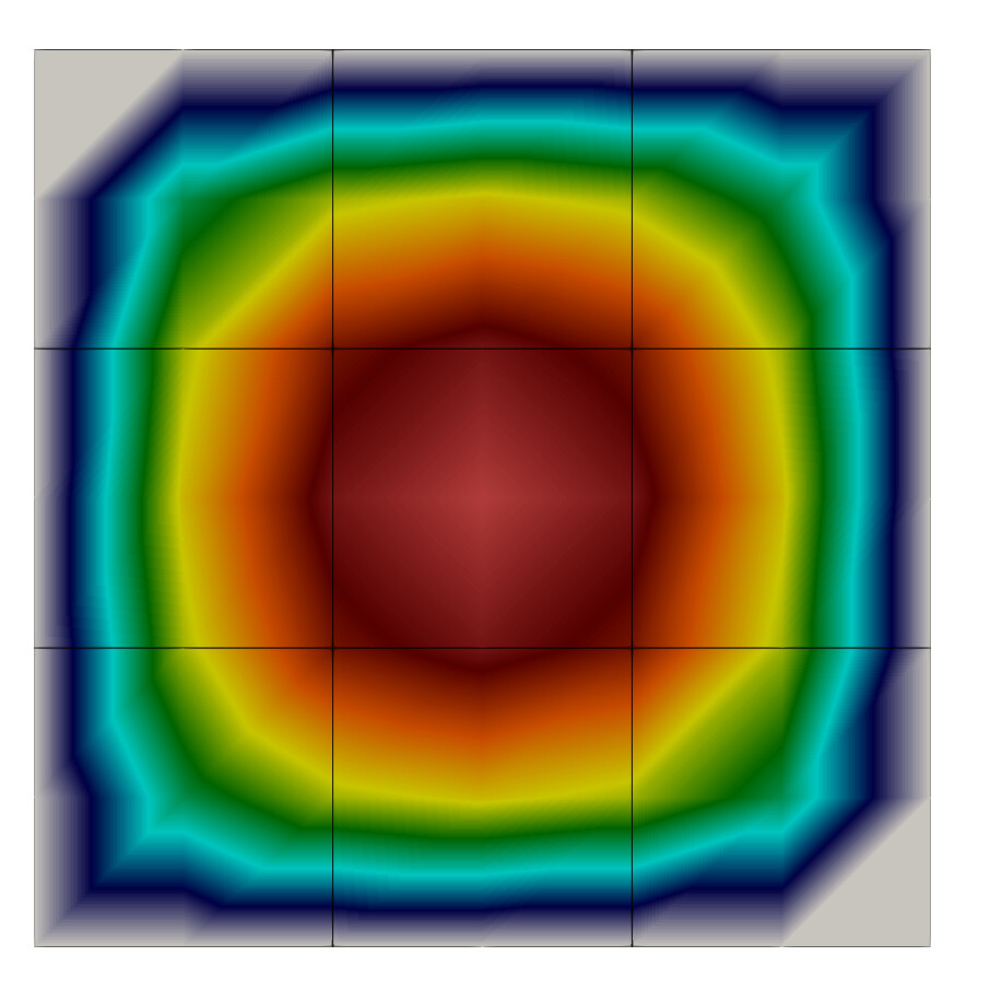
Here is a picture from above:

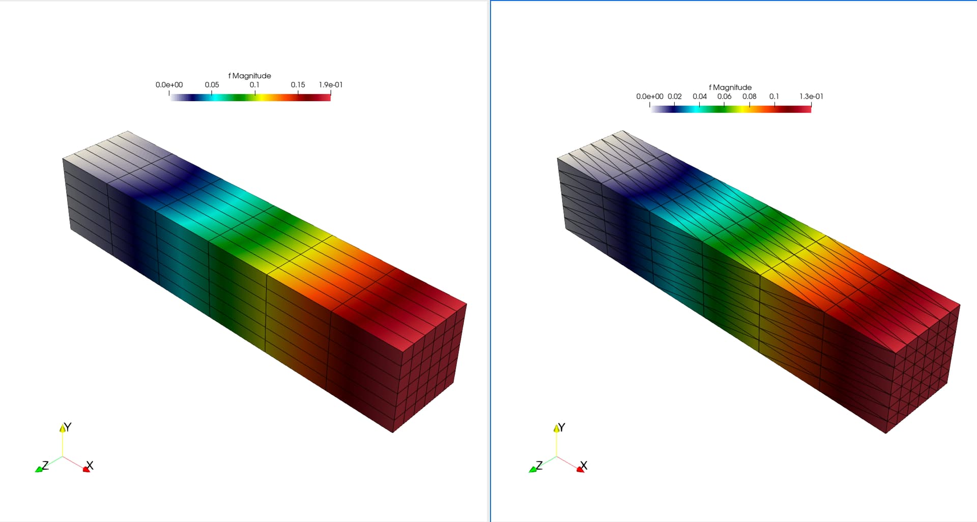
…and below:

By the way: the line

gmsh.model.geo.mesh.setTransfiniteSurface(1, "Alternate", [1, 2, 3, 4])

seems to be necessary to get a structured mesh, but the argument “Alternative” does not do anything, as we have quadrilaterals, and no triangles.

[Jesus_Vellojin]

Hi.

There is nothing wrong with your mesh. In fact, you can obtain the same results by using the built-in mesh:

msh= mesh.create_unit_square(MPI.COMM_WORLD, 4, 4, mesh.CellType.quadrilateral)

Since your space is P1, then the representation uses the DOF’s and a backend triangulation of the mesh. If you increase the scheme order, you will see the additional DOF’s over the mesh:

This is with P2

This is with P3

This could be very different is you use elements whose DOF’s are not nodes (like Raviart-Thomas or Nédelec where the DOF’s are normal moments):

NED1 on quads:

NED1 on triangles:

You can reproduce the above with (taken from https://github.com/FEniCS/dolfinx/blob/a9c5de0b370502baa111357a9063dcc2f83a1e15/python/demo/demo_pyvista.py#L232):

from mpi4py import MPI

# +
import numpy as np

from dolfinx.fem import Function, functionspace
from dolfinx.mesh import CellType, compute_midpoints, create_unit_cube, create_unit_square, meshtags
from dolfinx import mesh
import dolfinx

def plot_nedelec():
    msh = create_unit_square(comm=MPI.COMM_WORLD,nx=3,ny=3,
                                cell_type=mesh.CellType.triangle,
                                diagonal=mesh.DiagonalType.right_left)

    # msh = create_unit_square(comm=MPI.COMM_WORLD, nx=3, ny=3,
    #                          cell_type=mesh.CellType.quadrilateral)

    # Create a function space consisting of first order Nédélec (first kind)
    # elements and interpolate a vector-valued expression
    V = functionspace(msh, ("N1curl", 1))
    u = Function(V, dtype=np.float64)
    u.interpolate(lambda x: (x[1] ** 2, -x[0] * x[1]))

    # Exact visualisation of the Nédélec spaces requires a Lagrange or
    # discontinuous Lagrange finite element functions. Therefore, we
    # interpolate the Nédélec function into a first-order discontinuous
    # Lagrange space.
    gdim = msh.geometry.dim
    V0 = functionspace(msh, ("Discontinuous Lagrange", 2, (gdim,)))
    u0 = Function(V0, dtype=np.float64)
    u0.interpolate(u)

    
    with dolfinx.io.VTXWriter(MPI.COMM_WORLD, "uh_NED.bp", u0) as xf:
        xf.write(0.0)

plot_nedelec()

[renol-kth]

Thank you for your answer. This is interesting and counterintuitive for me.

What do you mean with “the representation uses the DOF’s and a backend triangulation of the mesh”? Do you mean, that even when choosing quadrilaterals, the dolfinx backend uses a triangulation (=triangle-shaped elements)?

I have never worked with quadrilaterals before, but what is strange to me is that when removing the line

gmsh.model.mesh.setRecombine(2, ps)

which in my understanding switches from quadrilaterals to triangles (and doubles the element number, as every quadrilateral is replaced by two triangles, but keeps the DOF number the same), I get almost the same solution.
Here with quads:

here with triangles:

the only difference seems to be the amplitude of the function, this visual overlap also appears for higher number of elements, e.g. 4 in each direction.

Could you help me get an intuition for this?

I understand how the basis functions look like, (e.g. degree 1 triangles and degree 1 quads). The Lagrange, degree 1 quadrilateral basis functions are nonlinear (and seemingly involve terms of degree 2, like e.g. xy if I am not mistaken?), while the triangle basis functions are linear.

Why do we get these visually similar solutions, even when using a completely different mesh shape and basis?

[Jesus_Vellojin]

What do you mean with “the representation uses the DOF’s and a backend triangulation of the mesh”? Do you mean, that even when choosing quadrilaterals, the dolfinx backend uses a triangulation (=triangle-shaped elements)?

Not the dolfinx backend, but Pyvista or Paraview. As far as I know, they triangulate everything in the backend even if you have a polygonal mesh. This is hardly noticeable in 2D, but you can observe it in 3D by performing a warp by vector with a sufficiently high factor.

I have never worked with quadrilaterals before, but what is strange to me is that when removing the line gmsh.model.mesh.setRecombine(2, ps) which in my understanding switches from quadrilaterals to triangles (and doubles the element number, as every quadrilateral is replaced by two triangles, but keeps the DOF number the same), I get almost the same solution.

As you said, the solutions looks similar, but they are not the same. The similarity comes from the location of the dofs, which is the same for both cases that are using Lagrange elements.

A similar case can be observed in the elasticity demo, where you can change tetrahedron by hexahedron for Lagrange elements and observe similar (but no same) results.

Could you help me get an intuition for this?
I understand how the basis functions look like, (e.g. degree 1 triangles and degree 1 quads). The Lagrange, degree 1 quadrilateral basis functions are nonlinear (and seemingly involve terms of degree 2, like e.g. xy if I am not mistaken?), while the triangle basis functions are linear.
Why do we get these visually similar solutions, even when using a completely different mesh shape and basis?

The lowest order quadrilateral element, is a bilinear element because it has the form (ax + b)(cy + d), and when restricted to an edge, they behave like the lowest order triangle element (see for example the book " Finite Elements and Fast Iterative Solvers" from Elman-Silvester). By looking some applications of FEM, like elasticity, you can find that the difference between both elements can be considerable in the study of slender structures, where the numerical locking plays a role.