Starting from
c_p \frac{\partial u }{\partial t} = k \nabla^2 u
in a one dimensional domain [0,1] where c_p and k are modeling two different materials:
k =
\begin{cases}
1 ~\text{if} ~x < 0.5\\
2.0 ~\text{else}
\end{cases}
c_p =
\begin{cases}
10^{-8} ~\text{if} ~x < 0.5\\
1.0 ~\text{else}
\end{cases}
I decided to refactor c_p to the right hand side such that
\frac{\partial u }{\partial t} = \frac{k} {c_p}\nabla^2 u
However, both solutions with FEniCS are different (this is a random time step, the trend is similar for all time steps):
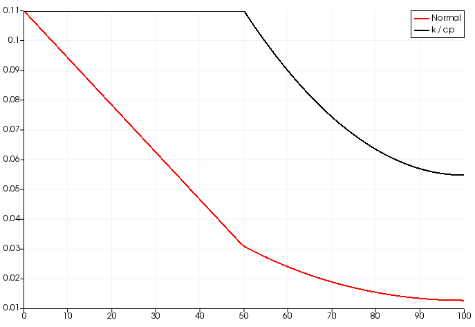
The one with c_p refactored shows a flat solution for x<0.5, whereas the original equation has a linear solution. This difference disappears when the material properties are homogeneous, which makes me think I might be committing some mistake in my finite element formulation. The code to run both examples is:
from fenics import *

cp_electrolyte = 1e-8
k_electrolyte = 1.0
k_electrode = 2.0
cp_electrode = 1.0
scan_rate = 1.0
output_dir = "./"

mesh = UnitIntervalMesh(100)

V = FunctionSpace(mesh, "CG", 1)
u, v = TrialFunction(V), TestFunction(V)

Vlimit = 1.0
tlimit = Vlimit / abs(scan_rate)


class Materials(UserExpression):
    def __init__(self, electrode, electrolyte, **kwargs):
        super().__init__(**kwargs)  # This part is new!
        self.electrolyte = electrolyte
        self.electrode = electrode

    def eval(self, values, x):
        if x[0] < 0.5:
            values[0] = self.electrolyte
        else:
            values[0] = self.electrode


k = Materials(k_electrode, k_electrolyte)
cp = Materials(cp_electrode, cp_electrolyte)

normal = False


def forward():

    dt_value = 1e-2
    dt = Constant(dt_value)
    u_n = Function(V)
    if normal:
        a = cp * u / dt * v * dx + k * \
            inner(Constant(1.0 / 2.0) * grad(u), grad(v)) * dx
        L = (
            cp * u_n / dt * v * dx
            - k * inner(Constant(1.0 / 2.0) * grad(u_n), grad(v)) * dx
        )
    else:
        a = u / dt * v * dx + k / cp * \
            inner(Constant(1.0 / 2.0) * grad(u), grad(v)) * dx
        L = (
            u_n / dt * v * dx
            - k / cp * inner(Constant(1.0 / 2.0) * grad(u_n), grad(v)) * dx
        )

    t = 0
    T = tlimit * 5
    n_steps = int(T / dt_value)

    bcval = Expression("t", t=t, degree=1)

    def Left(x, on_boundary):
        return x[0] < DOLFIN_EPS and on_boundary
    bc = DirichletBC(V, bcval, Left)

    u_sol = Function(V)
    if normal:
        output = "potential.pvd"
    else:
        output = "potential_ratio.pvd"
    potential_pvd = File(output)
    while t < T:
        solve(a == L, u_sol, bcs=bc)
        t += dt_value
        bcval.t = t
        potential_pvd << u_sol
        u_n.assign(u_sol)

    return u_n


u_n = forward()
Thanks