How are 2D manifolds immersed/embedded in 3D space handled in dolfinx?

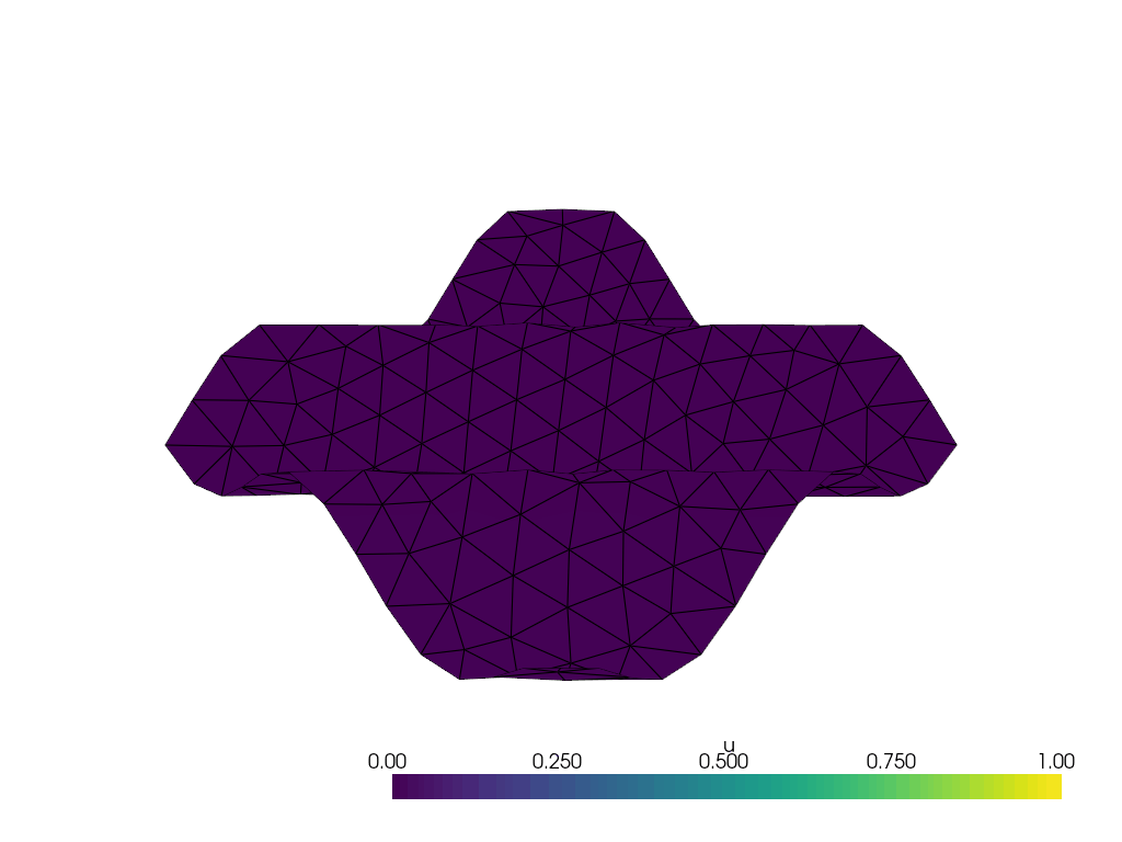
I have the following wavy 2D manifold defined by z = \frac{1}{10}\sin(10(x+y)) created with the following code with gmsh

##  Identify vertices, cells, and tags for each vertex/node
gmsh.initialize()
gmsh.model.add("wavy plate")

coords = [] # The x, y, z coordinates of all the nodes
nodes = [] # The tags of the corresponding nodes
tris = [] # The connectivities of the triangle elements (3 node tags per triangle) on the plate w/ topography
lin = [[], [], [], []] # The connectivities of the line elements on the 4 boundaries (2 node tags for each line element)
pnt = [tag(0, 0), tag(N, 0), tag(N, N), tag(0, N)] # The connectivities of the point elements on the 4 corners (1 node tag for each point element)
for i in range(N + 1):
    for j in range(N + 1):
        nodes.append(tag(i, j))
        coords.extend([
            float(i) / N,
            float(j) / N, 
            0.1 * np.sin(10 * float(i + j) / N)
        ])
        if i > 0 and j > 0:
            tris.extend([tag(i - 1, j - 1), tag(i, j - 1), tag(i - 1, j)])
            tris.extend([tag(i, j - 1), tag(i, j), tag(i - 1, j)])
        if (i == 0 or i == N) and j > 0:
            lin[3 if i == 0 else 1].extend([tag(i, j - 1), tag(i, j)])
        if (j == 0 or j == N) and i > 0:
            lin[0 if j == 0 else 2].extend([tag(i - 1, j), tag(i, j)])

# Create 4 discrete points for the 4 corners of the terrain surface:
for i in range(4):
    gmsh.model.addDiscreteEntity(dim = 0, tag = i + 1, boundary = []) # Create 4 corner points (dim = 0), with tags = {1,2,3,4}

# Set coordinates of each point (by tags = {1,2,3,4})
gmsh.model.setCoordinates(tag = 1, 
                          x = 0, 
                          y = 0, 
                          z = coords[3 * tag(0, 0) - 1])
gmsh.model.setCoordinates(tag = 2, 
                          x = coords[3 * tag(N, 0) - 1-2], 
                          y = coords[3 * tag(N, 0) - 1-1], 
                          z = coords[3 * tag(N, 0) - 1])
gmsh.model.setCoordinates(tag = 3, 
                          x = coords[3 * tag(N, N) - 1-2], 
                          y = coords[3 * tag(N, N) - 1-1], 
                          z = coords[3 * tag(N, N) - 1])
gmsh.model.setCoordinates(tag = 4, 
                          x = coords[3 * tag(0, N) - 1-2], 
                          y = coords[3 * tag(0, N) - 1-1], 
                          z = coords[3 * tag(0, N) - 1])

## Form Boundaries (by connecting 4 corner points)

for i in range(4): # 4 bounding curves
    gmsh.model.addDiscreteEntity(dim = 1, tag = i + 1, boundary = [i + 1, i + 2 if i < 3 else 1])# Creates 4 discrete bounding curves, with their boundary points
# Define (skeleton of) the surface
surface = gmsh.model.add_discrete_entity(dim = 2, tag = 1, boundary = [1,2,-3,-4]) # So far, surface just the 4 corners

## Add the nodes, points, lines, and cells to the surface

gmsh.model.mesh.addNodes(2, 1, nodes, coords) # Add nodes to surface
for i in range(4):
    # Type 15 for point elements:
    gmsh.model.mesh.addElementsByType(i + 1, 15, [], [pnt[i]]) # Add points to surface
    # Type 1 for 2-node line elements:
    gmsh.model.mesh.addElementsByType(i + 1, 1, [], lin[i]) # Add lines to surface
gmsh.model.mesh.addElementsByType(1, 2, [], tris) # Add elements/cells to surface (type 2 for 3-node triangular elements)

gmsh.model.mesh.reclassifyNodes() # Reclassify the nodes on the curves and the points
gmsh.model.mesh.createGeometry() # Create a geometry for the discrete curves and surfaces

gmsh.model.occ.synchronize() # Probably a good idea to synchronize before generating mesh

## Add Physical Group (important step for Dolfinx meshing) 

areas = gmsh.model.getEntities(dim=2) 
fluid_marker = 11 # What do you want the fluid marker to be named?
gmsh.model.addPhysicalGroup(areas[0][0], [areas[0][1]], fluid_marker) # Create the physical group
gmsh.model.setPhysicalName(areas[0][0], fluid_marker, "Fluid area")

## Mesh refinement

res = 1/10
gmsh.option.setNumber("Mesh.CharacteristicLengthMin", res)
gmsh.option.setNumber("Mesh.CharacteristicLengthMax", res)

## Generate mesh

gmsh.model.occ.synchronize()
gmsh.model.mesh.generate(2)

model_rank = 0
mesh, cell_tags, facet_tags = df.io.gmshio.model_to_mesh(gmsh.model, MPI.COMM_WORLD, model_rank)

I want to solve Poisson’s Equation, -\Delta u = f, on this manifold with Dirichlet boundary conditions. The variational form for Poisson’s Equation should still be

\int_\Omega \nabla u \cdot \nabla v d\Omega= \int_\Omega fv d\Omega

and for this to work, ufl.grad() needs to “understand” that the mesh is a wavy 2D manifold, not a flat x-y plane.

If it does not understand the context of the geometry of the mesh that the problem is being solved on, how would a problem like this be handled?

Hello @fea , I do not really see the issue here, theoretically. Since the global and the local coordinates, x and x’, are related through the wavy function, the grad is going to consider it.

Also, I guess your problem would now be a 2D manifold embedded in a 3D space. So, from an implementation point of view, BCs should be imposed in the 3D space (i.e., z direction as well), as your problem cannot be reduced to a 2D space.

1 Like

Hi, and thank you for your response! I hope it isn’t too much trouble to ask, but do you know of any manufactured solutions I could test for this manifold, or really any manifold that you have in mind? I don’t actually know how to define the Laplacian for this surface by hand, so whatever test solution, u, that I come up with, I don’t know what the resulting forcing term f, on the right hand side of the equation would be.

With a manufactured solution, I can make absolutely certain if Dolfinx and ufl have no issues with a problem like this, or if special treatment is required.

Forgot to include the tag function

# Helper function to return a node tag given two indices i and j:
def tag(i, j):
    return (N + 1) * i + j + 1

I’ve revived the code of Marie Rognes from 2013 (see supplementary material of: GMD - Automating the solution of PDEs on the sphere and other manifolds in FEniCS 1.2)

from mpi4py import MPI
import meshio
import ufl
import basix.ufl
import dolfinx
import scifem
import numpy as np

order = 2
tmp_data = meshio.dolfin.read("../hdiv-l2/meshes/sphere_ico3.xml")

mesh = dolfinx.mesh.create_mesh(
    comm=MPI.COMM_WORLD,
    cells=tmp_data.cells_dict["triangle"],
    x=tmp_data.points,
    e=ufl.Mesh(basix.ufl.element("Lagrange", "triangle", 1, shape=(3,))),
)

V_exact = dolfinx.fem.functionspace(mesh, ("Lagrange", order + 1, (mesh.geometry.dim,)))

# Define global normal
x = ufl.SpatialCoordinate(mesh)


S = dolfinx.fem.functionspace(mesh, ("DG", order, (mesh.geometry.dim,)))
L = dolfinx.fem.functionspace(mesh, ("DG", order))
V = dolfinx.fem.functionspace(mesh, ("Lagrange", order + 1))
R = scifem.create_real_functionspace(mesh)
W = ufl.MixedFunctionSpace(*(S, L, V, R))

(sigma, l, u, r) = ufl.TrialFunctions(W)
(w, gamma, v, t) = ufl.TestFunctions(W)

g = x[0] * x[1] * x[2]
up = ufl.as_vector((x[0], x[1], x[2]))


a = (
    ufl.dot(sigma, w)
    - ufl.dot(ufl.grad(u), w)
    - ufl.dot(w, up) * l
    + ufl.dot(sigma, ufl.grad(v))
    + gamma * ufl.dot(sigma, up)
    + u * t
    + r * v
) * ufl.dx
L_blocked = [
    ufl.ZeroBaseForm((w,)),
    ufl.ZeroBaseForm((gamma,)),
    -v * g * ufl.dx,
    ufl.ZeroBaseForm((t,)),
]

sigma_h = dolfinx.fem.Function(S)
l_h = dolfinx.fem.Function(L)
u_h = dolfinx.fem.Function(V)
r_h = dolfinx.fem.Function(R)
wh = (sigma_h, l_h, u_h, r_h)

petsc_options = {
    "ksp_type": "preonly",
    "pc_type": "lu",
    "pc_factor_mat_solver_type": "mumps",
    "ksp_error_if_not_converged": True,
    "ksp_monitor": None,
}


problem = dolfinx.fem.petsc.LinearProblem(
    ufl.extract_blocks(a),
    L_blocked,
    u=wh,
    bcs=[],
    petsc_options=petsc_options,
    petsc_options_prefix="mixed_poisson_",
    kind="mpi",
)
problem.solve()

with dolfinx.io.XDMFFile(mesh.comm, "new_mesh.xdmf", "w") as xdmf_file:
    xdmf_file.write_mesh(mesh)


with dolfinx.io.VTXWriter(mesh.comm, "u.bp", [u_h]) as vtx_writer:
    vtx_writer.write(0.0)

u_exact = -x[0] * x[1] * x[2] / 12
print(dolfinx.fem.assemble_scalar(dolfinx.fem.form(u_exact**2 * ufl.dx)))
L2_error_u = dolfinx.fem.form(ufl.inner(u_h - u_exact, u_h - u_exact) * ufl.dx)
print(
    "L2 error in u:",
    np.sqrt(mesh.comm.allreduce(dolfinx.fem.assemble_scalar(L2_error_u), op=MPI.SUM)),
)
with dolfinx.io.VTXWriter(mesh.comm, "u.bp", [u_h]) as vtx_writer:
    vtx_writer.write(0.0)


yields:
L2 error in u: 0.0004837339846541759

2 Likes

Could you provide the .xml file? I didn’t see it on the site hosting the article.

It’s in the supplementary material https://gmd.copernicus.org/articles/6/2099/2013/gmd-6-2099-2013-supplement.zip

1 Like

Hello, I have just made a demo with your geometry. I thought of creating a hyperelastic problem with sliding dirichlet BC on the bottom and left edges and stretching tractions on the top and right ones. This is the code:

import numpy as np
from mpi4py import MPI
import ufl
from dolfinx import fem, io, mesh, plot, default_scalar_type, log
from dolfinx.fem.petsc import NonlinearProblem
from dolfinx.nls.petsc import NewtonSolver
from dolfinx.io.gmshio import model_to_mesh
import gmsh
import pyvista
from petsc4py.PETSc import ScalarType  # type: ignore
import os

def create_domain(N):
    def tag(i, j):
        return (N + 1) * i + j + 1
    ##  Identify vertices, cells, and tags for each vertex/node
    gmsh.initialize()
    gmsh.model.add("wavy plate")

    coords = [] # The x, y, z coordinates of all the nodes
    nodes = [] # The tags of the corresponding nodes
    tris = [] # The connectivities of the triangle elements (3 node tags per triangle) on the plate w/ topography
    lin = [[], [], [], []] # The connectivities of the line elements on the 4 boundaries (2 node tags for each line element)
    pnt = [tag(0, 0), tag(N, 0), tag(N, N), tag(0, N)] # The connectivities of the point elements on the 4 corners (1 node tag for each point element)
    for i in range(N + 1):
        for j in range(N + 1):
            nodes.append(tag(i, j))
            coords.extend([
                float(i) / N,
                float(j) / N, 
                0.1 * np.sin(10 * float(i + j) / N)
            ])
            if i > 0 and j > 0:
                tris.extend([tag(i - 1, j - 1), tag(i, j - 1), tag(i - 1, j)])
                tris.extend([tag(i, j - 1), tag(i, j), tag(i - 1, j)])
            if (i == 0 or i == N) and j > 0:
                lin[3 if i == 0 else 1].extend([tag(i, j - 1), tag(i, j)])
            if (j == 0 or j == N) and i > 0:
                lin[0 if j == 0 else 2].extend([tag(i - 1, j), tag(i, j)])

    # Create 4 discrete points for the 4 corners of the terrain surface:
    for i in range(4):
        gmsh.model.addDiscreteEntity(dim = 0, tag = i + 1, boundary = []) # Create 4 corner points (dim = 0), with tags = {1,2,3,4}

    # Set coordinates of each point (by tags = {1,2,3,4})
    gmsh.model.setCoordinates(tag = 1, 
                            x = 0, 
                            y = 0, 
                            z = coords[3 * tag(0, 0) - 1])
    gmsh.model.setCoordinates(tag = 2, 
                            x = coords[3 * tag(N, 0) - 1-2], 
                            y = coords[3 * tag(N, 0) - 1-1], 
                            z = coords[3 * tag(N, 0) - 1])
    gmsh.model.setCoordinates(tag = 3, 
                            x = coords[3 * tag(N, N) - 1-2], 
                            y = coords[3 * tag(N, N) - 1-1], 
                            z = coords[3 * tag(N, N) - 1])
    gmsh.model.setCoordinates(tag = 4, 
                            x = coords[3 * tag(0, N) - 1-2], 
                            y = coords[3 * tag(0, N) - 1-1], 
                            z = coords[3 * tag(0, N) - 1])

    ## Form Boundaries (by connecting 4 corner points)

    for i in range(4): # 4 bounding curves
        gmsh.model.addDiscreteEntity(dim = 1, tag = i + 1, boundary = [i + 1, i + 2 if i < 3 else 1])# Creates 4 discrete bounding curves, with their boundary points
    # Define (skeleton of) the surface
    surface = gmsh.model.add_discrete_entity(dim = 2, tag = 1, boundary = [1,2,-3,-4]) # So far, surface just the 4 corners

    ## Add the nodes, points, lines, and cells to the surface

    gmsh.model.mesh.addNodes(2, 1, nodes, coords) # Add nodes to surface
    for i in range(4):
        # Type 15 for point elements:
        gmsh.model.mesh.addElementsByType(i + 1, 15, [], [pnt[i]]) # Add points to surface
        # Type 1 for 2-node line elements:
        gmsh.model.mesh.addElementsByType(i + 1, 1, [], lin[i]) # Add lines to surface
    gmsh.model.mesh.addElementsByType(1, 2, [], tris) # Add elements/cells to surface (type 2 for 3-node triangular elements)

    gmsh.model.mesh.reclassifyNodes() # Reclassify the nodes on the curves and the points
    gmsh.model.mesh.createGeometry() # Create a geometry for the discrete curves and surfaces

    gmsh.model.occ.synchronize() # Probably a good idea to synchronize before generating mesh

    ## Add Physical Group (important step for Dolfinx meshing) 

    areas = gmsh.model.getEntities(dim=2) 
    fluid_marker = 11 # What do you want the fluid marker to be named?
    gmsh.model.addPhysicalGroup(areas[0][0], [areas[0][1]], fluid_marker) # Create the physical group
    gmsh.model.setPhysicalName(areas[0][0], fluid_marker, "Fluid area")

    ## Mesh refinement

    res = 1/10
    gmsh.option.setNumber("Mesh.CharacteristicLengthMin", res)
    gmsh.option.setNumber("Mesh.CharacteristicLengthMax", res)

    ## Generate mesh

    gmsh.model.occ.synchronize()
    gmsh.model.mesh.generate(2)

    model_rank = 0
    return model_to_mesh(gmsh.model, MPI.COMM_WORLD, model_rank)

N = 100
domain, cell_tags, facet_tags = create_domain(N)
V = fem.functionspace(domain, ("Lagrange", 1, (domain.geometry.dim, )))

facets_top = mesh.locate_entities_boundary(
    domain,
    dim = domain.topology.dim - 1,
    marker = lambda x: np.logical_and(np.isclose(x[1], 1.0), np.logical_not(np.isclose(x[0], 0.0))),
)
facets_right = mesh.locate_entities_boundary(
    domain,
    dim = domain.topology.dim - 1,
    marker = lambda x: np.logical_and(np.isclose(x[0], 1.0), np.logical_not(np.isclose(x[1], 0.0))),
)
facets_bottom = mesh.locate_entities_boundary(
    domain,
    dim = domain.topology.dim - 1,
    marker = lambda x: np.isclose(x[1], 0.0),
)
facets_left = mesh.locate_entities_boundary(
    domain,
    dim = domain.topology.dim - 1,
    marker = lambda x: np.isclose(x[0], 0.0),
)
origin = mesh.locate_entities_boundary(
    domain,
    dim = domain.topology.dim - 2,
    marker = lambda x: np.logical_and(np.isclose(x[0], 0.0), np.isclose(x[1], 0.0)),
)
dofs_bottom = fem.locate_dofs_topological(V=V.sub(1), entity_dim=1, entities=facets_bottom)
dofs_left = fem.locate_dofs_topological(V=V.sub(0), entity_dim=1, entities=facets_left)
dofs_origin = fem.locate_dofs_topological(V=V.sub(2), entity_dim=0, entities=origin)
bcs = [fem.dirichletbc(value=ScalarType(0), dofs=dofs_left,   V=V.sub(0)),
       fem.dirichletbc(value=ScalarType(0), dofs=dofs_bottom, V=V.sub(1)),
       fem.dirichletbc(value=ScalarType(0), dofs=dofs_origin, V=V.sub(2))]

marked_facets = np.hstack([facets_top, facets_right])
marked_values = np.hstack([np.full_like(facets_top, 1), np.full_like(facets_right, 2)])
sorted_facets = np.argsort(marked_facets)
facet_tag = mesh.meshtags(domain, domain.topology.dim - 1, marked_facets[sorted_facets], marked_values[sorted_facets])

u = fem.Function(V)
v = ufl.TestFunction(V)

d = len(u)
I = ufl.variable(ufl.Identity(d))
F = ufl.variable(I + ufl.grad(u))
C = ufl.variable(F.T * F)
I1 = ufl.variable(ufl.tr(C))
J = ufl.variable(ufl.det(F))
Ic1 = I1/(J**(2/3))

E = default_scalar_type(1.0e4)
nu = default_scalar_type(0.3)
mu = fem.Constant(domain, E / (2 * (1 + nu)))
lmbda = fem.Constant(domain, E * nu / ((1 + nu) * (1 - 2 * nu)))
psi = (mu / 2) * (I1 - 3) - mu * ufl.ln(J) + (lmbda / 2) * (ufl.ln(J))**2
P = ufl.diff(psi, F)

metadata = {"quadrature_degree": 4}
ds = ufl.Measure('ds', domain=domain, subdomain_data=facet_tag, metadata=metadata)
dx = ufl.Measure("dx", domain=domain, metadata=metadata)
T_right = fem.Constant(domain, default_scalar_type((0, 0, 0)))
T_top = fem.Constant(domain, default_scalar_type((0, 0, 0)))
F = ufl.inner(ufl.grad(v), P) * dx - ufl.inner(v, T_right) * ds(2) - ufl.inner(v, T_top) * ds(1)


problem = NonlinearProblem(F, u, bcs)
solver = NewtonSolver(domain.comm, problem)
solver.atol = 1e-8
solver.rtol = 1e-8
solver.convergence_criterion = "incremental"


pyvista.start_xvfb()
plotter = pyvista.Plotter()
if not os.path.exists("deformation.gif"):
    open("deformation.gif", "x")
plotter.open_gif("deformation.gif", fps=20)

topology, cells, geometry = plot.vtk_mesh(u.function_space)
function_grid = pyvista.UnstructuredGrid(topology, cells, geometry)

values = np.zeros((geometry.shape[0], 3))
values[:, :len(u)] = u.x.array.reshape(geometry.shape[0], len(u))
function_grid["u"] = values
function_grid.set_active_vectors("u")

# Warp mesh by deformation
warped = function_grid.warp_by_vector("u", factor=1)
warped.set_active_vectors("u")

# Add mesh to plotter and visualize
plotter.add_mesh(warped, show_edges=True, lighting=False, clim=[0, 1])

# Compute magnitude of displacement to visualize in GIF
Vs = fem.functionspace(domain, ("Lagrange", 1))
magnitude = fem.Function(Vs)
us = fem.Expression(ufl.sqrt(sum([u[i]**2 for i in range(len(u))])), Vs.element.interpolation_points())
magnitude.interpolate(us)
warped["mag"] = magnitude.x.array


log.set_log_level(log.LogLevel.INFO)
tval0 = 25
for n in range(1, 101):
    print('New step...')
    T_top.value[1] = n * tval0
    T_right.value[0] = n * tval0
    num_its, converged = solver.solve(u)
    assert (converged)
    u.x.scatter_forward()
    print(f"Time step {n}, Number of iterations {num_its}, Load {n * tval0}")
    function_grid["u"][:, :len(u)] = u.x.array.reshape(geometry.shape[0], len(u))
    magnitude.interpolate(us)
    warped.set_active_scalars("mag")
    warped_n = function_grid.warp_by_vector(factor=1)
    warped.points[:, :] = warped_n.points
    warped.point_data["mag"][:] = magnitude.x.array
    plotter.update_scalar_bar_range([0, 1])
    plotter.write_frame()
plotter.close() 

The results are in the “deformation.gif” (I did it this way because I am currently having problems trying to visualize with pyvista while using WSL2). The latter looks like this:

deformation

EDIT: The picture is the other way round and for the warping function a more realistic approach could have been used, but I guess those are not relevant for the issue.

Just unzip the xml.gz files to xml.

1 Like

2 issues:

  1. petsc_options_prefix and kind when defining problem raise an error saying that these keywords do not exist. I don’t know if that’s a significant issue or not. I am on Dolfinx 0.9.0.

  2. after removing those 2 paramters, problem raises an error at defining self._A which is probably pertaining to input parameter a. It raises AttributeError: 'list' object has no attribute '_cpp_object'

Full error for issue 2 is

AttributeError                            Traceback (most recent call last)
Cell In[5], line 1
----> 1 problem = LinearProblem(
      2     ufl.extract_blocks(a),
      3     L_blocked,
      4     u=wh,
      5     bcs=[],
      6     petsc_options=petsc_options
      7 )
      8 problem.solve()
     10 with dolfinx.io.XDMFFile(mesh.comm, "new_mesh.xdmf", "w") as xdmf_file:

File ~/anaconda3/envs/fea2/lib/python3.13/site-packages/dolfinx/fem/petsc.py:788, in LinearProblem.__init__(self, a, L, bcs, u, petsc_options, form_compiler_options, jit_options)
    754 """Initialize solver for a linear variational problem.
    755 
    756 Args:
   (...)    780                                                                "mumps"})
    781 """
    782 self._a = _create_form(
    783     a,
    784     dtype=PETSc.ScalarType,
    785     form_compiler_options=form_compiler_options,
    786     jit_options=jit_options,
    787 )
--> 788 self._A = create_matrix(self._a)
    789 self._L = _create_form(
    790     L,
    791     dtype=PETSc.ScalarType,
    792     form_compiler_options=form_compiler_options,
    793     jit_options=jit_options,
    794 )
    795 self._b = create_vector(self._L)

File ~/anaconda3/envs/fea2/lib/python3.13/site-packages/dolfinx/fem/petsc.py:176, in create_matrix(a, mat_type)
    160 """Create a PETSc matrix that is compatible with a bilinear form.
    161 
    162 Note:
   (...)    173     A PETSc matrix with a layout that is compatible with ``a``.
    174 """
    175 if mat_type is None:
--> 176     return _cpp.fem.petsc.create_matrix(a._cpp_object)
    177 else:
    178     return _cpp.fem.petsc.create_matrix(a._cpp_object, mat_type)

AttributeError: 'list' object has no attribute '_cpp_object'

the code is made to work with DOLFINx nightly, where the solver API is massively improved. It can for instance be accessed through the docker images.

I create and run my code in Jupyter Notebook through Anaconda installed on Ubuntu via WSL2. I have not installed the docker engine into Ubuntu on either my root or in my virtual environment, and I don’t know how to use it in general or how to integrate this nightly version once it has been pulled into my particular setup. Would it be too much trouble for you to modify your code to work with regular Dolfinx to get around the lack of this API I’m assuming is causing the problem? Or would it end up being less troublesome figuring out how to install the nightly version?

What was the definition for the analytic solution that you were comparing your approximate solution to?

With the following modifications the code should run on 0.9.0


a = (
    ufl.dot(sigma, w)
    - ufl.dot(ufl.grad(u), w)
    - ufl.dot(w, up) * l
    + ufl.dot(sigma, ufl.grad(v))
    + gamma * ufl.dot(sigma, up)
    + u * t
    + r * v
) * ufl.dx
L_blocked = [
    ufl.inner(
        dolfinx.fem.Constant(
            mesh, np.zeros(mesh.geometry.dim, dtype=dolfinx.default_scalar_type)
        ),
        w,
    )
    * ufl.dx,
    ufl.inner(dolfinx.fem.Constant(mesh, 0.0), gamma) * ufl.dx,
    -v * g * ufl.dx,
    ufl.inner(dolfinx.fem.Constant(mesh, 0.0), t) * ufl.dx,
]

sigma_h = dolfinx.fem.Function(S)
l_h = dolfinx.fem.Function(L)
u_h = dolfinx.fem.Function(V)
r_h = dolfinx.fem.Function(R)
wh = (sigma_h, l_h, u_h, r_h)

petsc_options = {
    "ksp_type": "preonly",
    "pc_type": "lu",
    "pc_factor_mat_solver_type": "mumps",
    "ksp_error_if_not_converged": True,
    "ksp_monitor": None,
}

from petsc4py import PETSc

a_comp = dolfinx.fem.form(ufl.extract_blocks(a))
A = dolfinx.fem.petsc.assemble_matrix_block(a_comp)
A.assemble()
b = dolfinx.fem.petsc.assemble_vector_block(dolfinx.fem.form(L_blocked), a_comp)

ksp = PETSc.KSP().create(mesh.comm)
ksp.setOperators(A)
opts = PETSc.Options()
for key, value in petsc_options.items():
    opts[key] = value
ksp.setFromOptions()

uh_vec = b.duplicate()
ksp.solve(b, uh_vec)

offset = 0
x_array = uh_vec.getArray(readonly=True)
for var in wh:
    size_local = var.x.petsc_vec.getLocalSize()
    var.x.petsc_vec.array[:] = x_array[offset : offset + size_local]
    var.x.petsc_vec.ghostUpdate(
        addv=PETSc.InsertMode.INSERT, mode=PETSc.ScatterMode.FORWARD
    )
    offset += size_local

Oh, well, I did not compare the computed approximated solution to the exact solution of the hyperelastic problem on your 2D manifold. It was just a quick piece of code showing that 2D manifolds embedded in 3D spaces are treated as any other type of problem (e.g., 3D manifolds in 3D spaces, etc.).

I’ve not seen KSP before, but its description says it manages the linear solvers in PETSc, so probably ksp is in place of the usual problem = dolfinx.fem.petsc.LinearProblem(). Also, I don’t understand how this works, but running ksp.solve(b, uh_vec) not only gives uh_vec which is the solution vector, but it also seems to populate u_h which is our solution because running

print(dolfinx.fem.assemble_scalar(dolfinx.fem.form(u_exact**2 * ufl.dx)))
L2_error_u = dolfinx.fem.form(ufl.inner(u_h - u_exact, u_h - u_exact) * ufl.dx)
print(
    "L2 error in u:",
    np.sqrt(mesh.comm.allreduce(dolfinx.fem.assemble_scalar(L2_error_u), op=MPI.SUM)),
)

still works and outputs the same L2. Additionally, I also don’t understand what the purpose and outcome of the lines

offset = 0
x_array = uh_vec.getArray(readonly=True)
for var in wh:
    size_local = var.x.petsc_vec.getLocalSize()
    var.x.petsc_vec.array[:] = x_array[offset : offset + size_local]
    var.x.petsc_vec.ghostUpdate(
        addv=PETSc.InsertMode.INSERT, mode=PETSc.ScatterMode.FORWARD
    )
    offset += size_local

are.

Yeah, this looks like its own can of worms to parse through and figure out, so figuring out how to use the nightly version as it allows me to keep things closer to the tutorials might be worth it after all. Can it be installed for my particular setup?

Oh okay, now I understand. There might have been a misunderstanding, I was looking for a manufactured solution to test i.e. a problem in which the solution is known, and we attempt to find an approximate solution to compare it to. But if this problem you’ve shown accomplishes to illustrate that it handles this manifold without issue, then that’s good enough for me.

To learn about PETSc, see for instance

The second set of lines assigns the solution from uh_vec to the functions

Docker is the easiest way to go for the nightly branch. Spack is another alternative.

If one want’s to work with H-div conforming spaces on orientable manifolds, a slight workaround is needed, see:

1 Like

Oh, thank you very much for the information! It is always good to know this kind of workarounds.