If we try to solve the Navier stokes equation for a rectangle:
We can generate the rectangle as follows:
import numpy as np
import gmsh
from dolfinx.io.gmshio import model_to_mesh
from mpi4py import MPI

A = np.array([0,0])
B = np.array([3,0])
C = np.array([3,1])
D = np.array([0,1])

gmsh.initialize()
mesh_size = 0.1
point_1 = gmsh.model.geo.add_point(A[0],A[1], 0, mesh_size)
point_2 = gmsh.model.geo.add_point(B[0],B[1], 0, mesh_size)
point_3 = gmsh.model.geo.add_point(C[0],C[1], 0, mesh_size)
point_4 = gmsh.model.geo.add_point(D[0],D[1], 0, mesh_size)

line_1 = gmsh.model.geo.add_line(point_1, point_2)
line_2 = gmsh.model.geo.add_line(point_2, point_3)
line_3 = gmsh.model.geo.add_line(point_3, point_4)
line_4 = gmsh.model.geo.add_line(point_4, point_1)

curve_loop    = gmsh.model.geo.add_curve_loop([line_1,line_2,line_3,line_4])
plane_surface = gmsh.model.geo.add_plane_surface([curve_loop])

gmsh.model.geo.synchronize()

gmsh.model.addPhysicalGroup(1, [line_1,line_2,line_3,line_4], name = "added physical curve")

gmsh.model.addPhysicalGroup(2, [plane_surface], name = "added physical surface")

gmsh.model.mesh.generate()

mesh, cell_tags, facet_tags = model_to_mesh(gmsh.model, MPI.COMM_WORLD, 0,gdim=2)

gmsh.finalize()
You can draw the mesh by:
import pyvista
from dolfinx import plot

topology, cell_types, geometry_for_plotting = plot.create_vtk_mesh(mesh, 2)

grid = pyvista.UnstructuredGrid(topology, cell_types, geometry_for_plotting)

pyvista.set_jupyter_backend("pythreejs")

plotter = pyvista.Plotter()
plotter.add_mesh(grid, show_edges=True)
plotter.view_xy()

if not pyvista.OFF_SCREEN:
    plotter.show()
else:
    pyvista.start_xvfb()
    figure = plotter.screenshot("fundamentals_mesh.png")
Notice that A B C and D are corner points and we can define the no slip and inflow/ outflow conditions as follows:
from ufl import  VectorElement,FiniteElement
from dolfinx.fem import FunctionSpace,locate_dofs_geometrical,dirichletbc
from petsc4py import PETSc

v_cg2 = VectorElement("CG", mesh.ufl_cell(), 2)
s_cg1 = FiniteElement("CG", mesh.ufl_cell(), 1)
V = FunctionSpace(mesh, v_cg2)
Q = FunctionSpace(mesh, s_cg1)


def walls(x):

    return np.logical_or(np.isclose(x[1],A[1]), np.isclose(x[1],C[1]))

wall_dofs = locate_dofs_geometrical(V, walls)
u_noslip = np.array((0,) * mesh.geometry.dim, dtype=PETSc.ScalarType)
bc_noslip = dirichletbc(u_noslip, wall_dofs, V)

inflow_pressure = 1
def inflow(x):
    return np.isclose(x[0], A[0])
inflow_dofs = locate_dofs_geometrical(Q, inflow)
bc_inflow = dirichletbc(PETSc.ScalarType(inflow_pressure), inflow_dofs, Q)

def outflow(x):
    return np.isclose(x[0], C[0])
outflow_dofs = locate_dofs_geometrical(Q, outflow)
bc_outflow = dirichletbc(PETSc.ScalarType(0), outflow_dofs, Q)
bcu = [bc_noslip]
bcp = [bc_inflow, bc_outflow]
Here, I used the coordinates of A and C to determine the locations of walls (used from tutorial)
However, now suppose we have slanted domain edges as below:
A = np.array([0,0])
B = np.array([2,1])
C = np.array([2,3])
D = np.array([-1,2])

gmsh.initialize()
mesh_size = 0.1
point_1 = gmsh.model.geo.add_point(A[0],A[1], 0, mesh_size)
point_2 = gmsh.model.geo.add_point(B[0],B[1], 0, mesh_size)
point_3 = gmsh.model.geo.add_point(C[0],C[1], 0, mesh_size)
point_4 = gmsh.model.geo.add_point(D[0],D[1], 0, mesh_size)

line_1 = gmsh.model.geo.add_line(point_1, point_2)
line_2 = gmsh.model.geo.add_line(point_2, point_3)
line_3 = gmsh.model.geo.add_line(point_3, point_4)
line_4 = gmsh.model.geo.add_line(point_4, point_1)

curve_loop    = gmsh.model.geo.add_curve_loop([line_1,line_2,line_3,line_4])
plane_surface = gmsh.model.geo.add_plane_surface([curve_loop])

gmsh.model.geo.synchronize()

gmsh.model.addPhysicalGroup(1, [line_1,line_2,line_3,line_4], name = "added physical curve")

gmsh.model.addPhysicalGroup(2, [plane_surface], name = "added physical surface")

gmsh.model.mesh.generate()

mesh, cell_tags, facet_tags = model_to_mesh(gmsh.model, MPI.COMM_WORLD, 0,gdim=2)

gmsh.finalize()
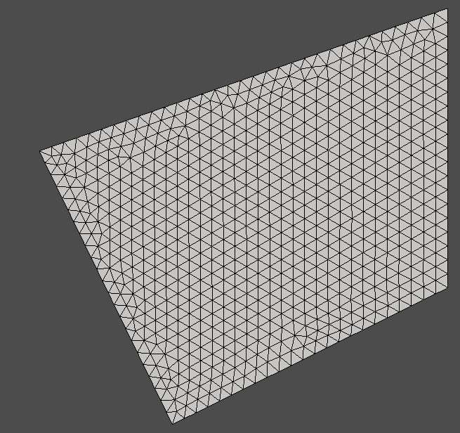
We can no longer use the coordinates A,B,C or D to define the boundary.
So, may I please know what can we do in a situation like this…?
In my actual code I have so many edges and writing down straight line equations for each edge is impossible…