Hi, I have an elastic body with a complex shape and I want to see how big the deformation is at different points when a force is applied at a surface.
The body looks like this plate with two islands and a connecting bridge:
(visible in the picture and the bottom since I can only upload one image. Please ignore the arrows for now)
I apply a set force on the surface on the bridge (in red in the bottom image) that pushes into the material and look how big the deformation is in the material.
I while trying to reuse the code of fenics-tutorial/ft06_elasticity.py at master · hplgit/fenics-tutorial · GitHub I got this:
import fenics as fx
import mshr

#define the mesh in µm
whole = mshr.Box(fx.Point(-100, -100, 0), fx.Point(100, 100, 10))
box1 = mshr.Box(fx.Point(20, 20, 10), fx.Point(60, -20, 0))
box2 = mshr.Box(fx.Point(-20, 20, 10), fx.Point(-60, -20, 0))
channel = mshr.Box(fx.Point(-20, 3.5, 10), fx.Point(20, -3.5, 0))

domain = whole - box1 -box2 -channel
mesh = mshr.generate_mesh(domain, 128)

# unscaled variables
E = 300
G = 70
mu = G
lambda_ = G*(E-2*G) / (3*G - E)

V = fx.VectorFunctionSpace(mesh, 'Lagrange', 1)

tol = 1E-14
def boundary(x, on_boundary):
    res = False
    if fx.near(x[2], 0, tol):
        res = True
    if fx.near(x[0], -100, tol) or fx.near(x[0], 100, tol):
        res = True
    if fx.near(x[1], -100, tol) or fx.near(x[1], 100, tol):
        res = True
    return res

bc = fx.DirichletBC(V, fx.Constant((0, 0, 0)), boundary)

# Define strain and stress

def epsilon(u):
    return 0.5*(fx.nabla_grad(u) + fx.nabla_grad(u).T)
    #return sym(nabla_grad(u))

def sigma(u):
    #return lambda_*fx.nabla_div(u)*fx.Identity(d) + 2*mu*epsilon(u)
    return lambda_* fx.div(u) * fx.Identity(d) + 2*mu*epsilon(u)


# Define variational problem
u = fx.TrialFunction(V)
d = u.geometric_dimension()  # space dimension
v = fx.TestFunction(V)

# force is (0,1k,0) at the bridge surface (like 0.5 deep into the mesh) and (0,0,0) everywhere else
f = fx.Expression(('0', 'x[0]>=-20 && x[0]<=20 && x[1]>=3 && x[1]<=4 ? 1000 : 0', '0'), element = V.ufl_element())

T = fx.Constant((0, 0, 0))
a = fx.inner(sigma(u), epsilon(v))*fx.dx
L = fx.dot(f, v)*fx.dx + fx.dot(T, v)*fx.ds

# Compute solution
u = fx.Function(V)
fx.solve(a == L, u, bc, solver_parameters={'linear_solver':'mumps'})

fx.File('dumbbell/displacement.pvd') << u
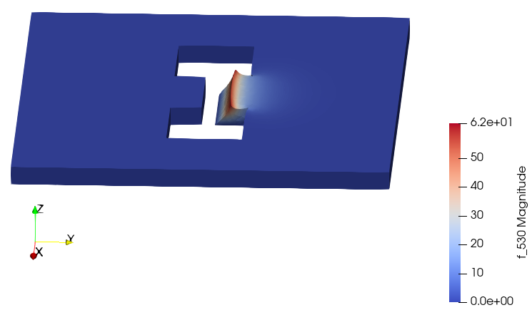
But when I look at it in paraview I get rather strange deformation glyphs like this while I would expect the bridge to just be pushed in y direction and almost not at all in z.

Is my code wrong or is that really the expected deformation?
And how to I read out the deformation on a given plane inside my body like the z=5 plane?
Sorry for the lengthy post and thanks in advance!