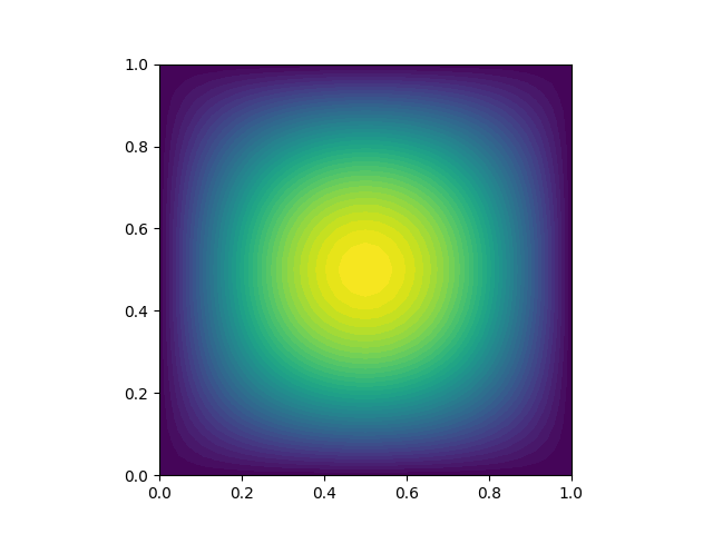
HI all. I run demo_biharmonic.py but I didn’t get the same image as they given in biharmonic_u.png . What I got is below. I open it in paraview by using command paraview biharmonic.pvd but didn’t get the result. Also the L2 error goes increasing as I fine the mesh.The code is given below.On taking mesh = UnitSquareMesh(2,2) I got 0.284522 and on taking mesh = UnitSquareMesh(4,4) I got 0.401958. Our error must decrease with finer refinement but it increases as we do the mesh finer. Kindly help me regarding the same. Thanku.
# Biharmonic equation
# ===================
#
# This demo is implemented in a single Python file,
# :download:`demo_biharmonic.py`, which contains both the variational
# forms and the solver.
#
# This demo illustrates how to:
#
# * Solve a linear partial differential equation
# * Use a discontinuous Galerkin method
# * Solve a fourth-order differential equation
#
# The solution for :math:`u` in this demo will look as follows:
#
# .. image:: biharmonic_u.png
#     :scale: 75 %
#
#
# Equation and problem definition
# -------------------------------
#
# The biharmonic equation is a fourth-order elliptic equation. On the
# domain :math:`\Omega \subset \mathbb{R}^{d}`, :math:`1 \le d \le 3`,
# it reads
#
# .. math::
#    \nabla^{4} u = f \quad {\rm in} \ \Omega,
#
# where :math:`\nabla^{4} \equiv \nabla^{2} \nabla^{2}` is the
# biharmonic operator and :math:`f` is a prescribed source term. To
# formulate a complete boundary value problem, the biharmonic equation
# must be complemented by suitable boundary conditions.
#
# Multiplying the biharmonic equation by a test function and integrating
# by parts twice leads to a problem second-order derivatives, which
# would requires :math:`H^{2}` conforming (roughly :math:`C^{1}`
# continuous) basis functions.  To solve the biharmonic equation using
# Lagrange finite element basis functions, the biharmonic equation can
# be split into two second-order equations (see the Mixed Poisson demo
# for a mixed method for the Poisson equation), or a variational
# formulation can be constructed that imposes weak continuity of normal
# derivatives between finite element cells.  The demo uses a
# discontinuous Galerkin approach to impose continuity of the normal
# derivative weakly.
#
# Consider a triangulation :math:`\mathcal{T}` of the domain
# :math:`\Omega`, where the set of interior facets is denoted by
# :math:`\mathcal{E}_h^{\rm int}`.  Functions evaluated on opposite
# sides of a facet are indicated by the subscripts ':math:`+`' and
# ':math:`-`'.  Using the standard continuous Lagrange finite element
# space
#
# .. math::
#     V = \left\{v \in H^{1}_{0}(\Omega)\,:\, v \in P_{k}(K) \ \forall \ K \in \mathcal{T} \right\}
#
# and considering the boundary conditions
#
# .. math::
#    u            &= 0 \quad {\rm on} \ \partial\Omega \\
#    \nabla^{2} u &= 0 \quad {\rm on} \ \partial\Omega
#
# a weak formulation of the biharmonic problem reads: find :math:`u \in
# V` such that
#
# .. math::
#   a(u,v)=L(v) \quad \forall \ v \in V,
#
# where the bilinear form is
#
#
# .. math::
#    a(u, v) = \sum_{K \in \mathcal{T}} \int_{K} \nabla^{2} u \nabla^{2} v \, {\rm d}x \
#   +\sum_{E \in \mathcal{E}_h^{\rm int}}\left(\int_{E} \frac{\alpha}{h_E} [\!\![ \nabla u ]\!\!] [\!\![ \nabla v ]\!\!] \, {\rm d}s
#   - \int_{E} \left<\nabla^{2} u \right>[\!\![ \nabla v ]\!\!]  \, {\rm d}s
#   - \int_{E} [\!\![ \nabla u ]\!\!]  \left<\nabla^{2} v \right>  \, {\rm d}s\right)
#
# and the linear form is
#
# .. math::
#   L(v) = \int_{\Omega} fv \, {\rm d}x
#
# Furthermore, :math:`\left< u \right> = \frac{1}{2} (u_{+} + u_{-})`,
# :math:`[\!\![ w ]\!\!]  = w_{+} \cdot n_{+} + w_{-} \cdot n_{-}`,
# :math:`\alpha \ge 0` is a penalty parameter and :math:`h_E` is a
# measure of the cell size.
#
# The input parameters for this demo are defined as follows:
#
# * :math:`\Omega = [0,1] \times [0,1]` (a unit square)
# * :math:`\alpha = 8.0` (penalty parameter)
# * :math:`f = 4.0 \pi^4\sin(\pi x)\sin(\pi y)` (source term)
#
#
# Implementation
# --------------
#
# This demo is implemented in the :download:`demo_biharmonic.py` file.
#
# First, the necessary modules are imported::

import matplotlib.pyplot as plt
from dolfin import *

# Next, some parameters for the form compiler are set::

# Optimization options for the form compiler
parameters["form_compiler"]["cpp_optimize"] = True
parameters["form_compiler"]["optimize"] = True

# A mesh is created, and a quadratic finite element function space::

# Make mesh ghosted for evaluation of DG terms
parameters["ghost_mode"] = "shared_facet"

# Create mesh and define function space
mesh = UnitSquareMesh(4,4)
V = FunctionSpace(mesh, "CG", 2)

# A subclass of :py:class:`SubDomain <dolfin.cpp.SubDomain>`,
# ``DirichletBoundary`` is created for later defining the boundary of
# the domain::

# Define Dirichlet boundary
class DirichletBoundary(SubDomain):
    def inside(self, x, on_boundary):
        return on_boundary

# A subclass of :py:class:`Expression
# <dolfin.functions.expression.Expression>`, ``Source`` is created for
# the source term :math:`f`::

class Source(UserExpression):
    def eval(self, values, x):
        values[0] = 4.0*pi**4*sin(pi*x[0])*sin(pi*x[1])

# The Dirichlet boundary condition is created::

# Define boundary condition
u0 = Constant(0.0)
bc = DirichletBC(V, u0, DirichletBoundary())

# On the finite element space ``V``, trial and test functions are
# created::

# Define trial and test functions
u = TrialFunction(V)
v = TestFunction(V)

# A function for the cell size :math:`h` is created, as is a function
# for the average size of cells that share a facet (``h_avg``).  The UFL
# syntax ``('+')`` and ``('-')`` restricts a function to the ``('+')``
# and ``('-')`` sides of a facet, respectively. The unit outward normal
# to cell boundaries (``n``) is created, as is the source term ``f`` and
# the penalty parameter ``alpha``. The penalty parameters is made a
# :py:class:`Constant <dolfin.functions.constant.Constant>` so that it
# can be changed without needing to regenerate code. ::

# Define normal component, mesh size and right-hand side
h = CellDiameter(mesh)
h_avg = (h('+') + h('-'))/2.0
n = FacetNormal(mesh)
f = Source(degree=2)

# Penalty parameter
alpha = Constant(8.0)

# The bilinear and linear forms are defined::

# Define bilinear form
a = inner(div(grad(u)), div(grad(v)))*dx \
  - inner(avg(div(grad(u))), jump(grad(v), n))*dS \
  - inner(jump(grad(u), n), avg(div(grad(v))))*dS \
  + alpha/h_avg*inner(jump(grad(u),n), jump(grad(v),n))*dS

# Define linear form
L = f*v*dx

# A :py:class:`Function <dolfin.functions.function.Function>` is created
# to store the solution and the variational problem is solved::

# Solve variational problem
u = Function(V)
solve(a == L, u, bc)

error_L2 = errornorm(u0, u, 'L2')
print('error_L2  =', error_L2)

# The computed solution is written to a file in VTK format and plotted to
# the screen. ::

# Save solution to file
file = File("biharmonic.pvd")
file << u

# Plot solution
plot(u)
plt.show()