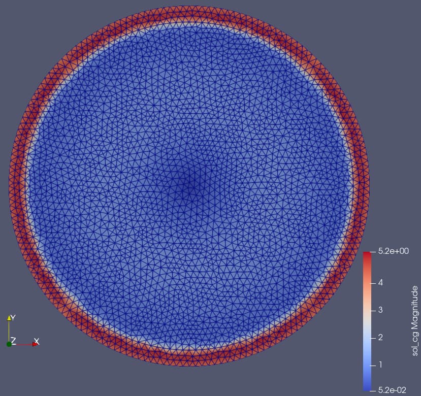
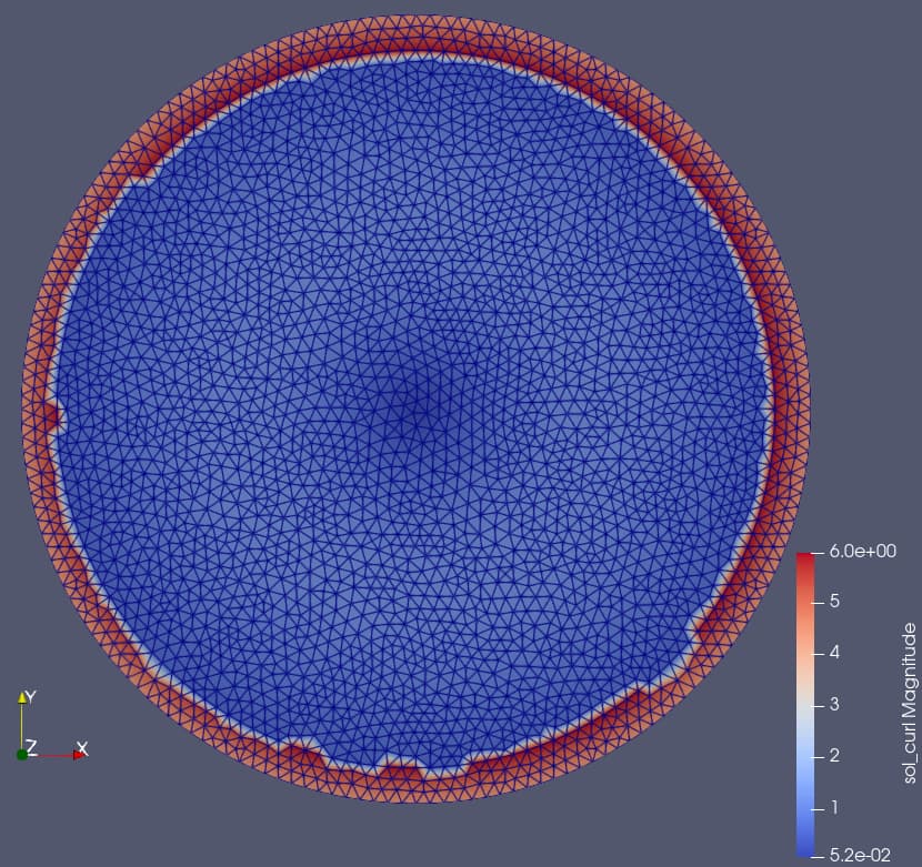
I’m using DG0 elements to assign materials to mesh regions like in this example. When I use these material DG0 functions together with Ncurl elements I get ragged field on the material boundary like in the picture below (compared to the vector CG elements). When using this function in further calculations errors pile up resulting in unstable solution and wrong results.
What can I do to fix this behaviour?
PS. I didn’t experience this behaviour in Dolfin
Gmsh model mesh.geo:
Geometry.OCCTargetUnit = "M";

r1 = 1;
r2 = 1.1;
dx1 = 0.5;
dy1 = 0.5;
dx2 = 0.5;
dy2 = 0.5;
mesh1 = 0.04;
mesh2 = 0.04;

p0 = newp; Point(p0) = {dx1,dy1,0,mesh1};
p1 = newp; Point(p1) = {r1+dx1,dy1,0,mesh1};
p2 = newp; Point(p2) = {dx1,r1+dy1,0,mesh1};
p3 = newp; Point(p3) = {-r1+dx1,dy1,0,mesh1};
p4 = newp; Point(p4) = {dx1,-r1+dy1,0,mesh1};
l1 = newl; Circle(l1) = {p1,p0,p2};
l2 = newl; Circle(l2) = {p2,p0,p3};
l3 = newl; Circle(l3) = {p3,p0,p4};
l4 = newl; Circle(l4) = {p4,p0,p1};
ll1 = newll; Line loop(ll1) = {l1,l2,l3,l4};
s1 = news; Surface(s1) = {ll1};

p00 = newp; Point(p00) = {dx2,dy2,0,mesh2};
p10 = newp; Point(p10) = {r2+dx2,dy2,0,mesh2};
p20 = newp; Point(p20) = {dx2,r2+dy2,0,mesh2};
p30 = newp; Point(p30) = {-r2+dx2,dy2,0,mesh2};
p40 = newp; Point(p40) = {dx2,-r2+dy2,0,mesh2};
l10 = newl; Circle(l10) = {p10,p00,p20};
l20 = newl; Circle(l20) = {p20,p00,p30};
l30 = newl; Circle(l30) = {p30,p00,p40};
l40 = newl; Circle(l40) = {p40,p00,p10};
ll10 = newll; Line loop(ll10) = {l10,l20,l30,l40};
s10 = news; Surface(s10) = {ll10, ll1};

Physical Surface(1) = {s1};
Physical Surface(2) = {s10};
Generate gmsh mesh mesh.msh using command gmsh mesh.geo -2
DolfinX code:
import dolfinx
import dolfinx.io
import ufl
import numpy as np
from mpi4py import MPI


def convert_msh(input_file: str, output_file: str,
                cell_type="triangle", cell_data_tag="gmsh:physical"):
    import meshio

    msh = meshio.read(input_file)
    msh.prune_z_0()
    msh.remove_orphaned_nodes()
    cells = msh.get_cells_type(cell_type)
    regions = msh.get_cell_data(cell_data_tag, cell_type)
    out_mesh = meshio.Mesh(points=msh.points,
                           cells={cell_type: cells},
                           cell_data={"regions": [regions]})
    meshio.write(output_file, out_mesh, file_format="xdmf")

# convert mesh to dolfinx
convert_msh("mesh.msh", "mesh.xdmf")

with dolfinx.io.XDMFFile(MPI.COMM_WORLD, "mesh.xdmf", "r") as xdmf:
    mesh = xdmf.read_mesh(name="Grid")
    subdomains = xdmf.read_meshtags(mesh, name="Grid")

# assign material
V = dolfinx.FunctionSpace(mesh, ("Discontinuous Lagrange", 0))
mat = dolfinx.Function(V)
mat.name = "material"
with mat.vector.localForm() as loc:
    loc.set(0)
    cells = subdomains.indices[subdomains.values == 2]
    loc.setValues(cells, np.full(cells.size, 1))

H1 = ufl.FiniteElement("Lagrange", mesh.ufl_cell(), 2)
Hvec = ufl.VectorElement(H1, dim=2)
Hcurl = ufl.FiniteElement("Nedelec 1st kind H(curl)", mesh.ufl_cell(), 2)

# source function
V = dolfinx.FunctionSpace(mesh, H1)
f = dolfinx.Function(V)
f.name = "source"
f.interpolate(lambda x: np.exp(- (x[0] - 0.5)**2 / (2 * 0.5**2)
                          - (x[1] - 0.5)**2 / (2 * 0.5**2)))

# CG solution
V = dolfinx.FunctionSpace(mesh, Hvec)
sol_cg = dolfinx.Function(V)
sol_cg.name = "sol_cg"
u, v = ufl.TrialFunction(V), ufl.TestFunction(V)
a = ufl.inner(u, v) * ufl.dx
L = ufl.inner(ufl.grad(f) + 10 * mat * ufl.grad(f), v) * ufl.dx
dolfinx.fem.LinearProblem(a, L, u=sol_cg).solve()

# Hcurl solution
V = dolfinx.FunctionSpace(mesh, Hcurl)
sol_curl = dolfinx.Function(V)
sol_curl.name = "sol_curl"
u, v = ufl.TrialFunction(V), ufl.TestFunction(V)
a = ufl.inner(u, v) * ufl.dx
L = ufl.inner(ufl.grad(f) + 10 * mat * ufl.grad(f), v) * ufl.dx
dolfinx.fem.LinearProblem(a, L, u=sol_curl).solve()

with dolfinx.io.XDMFFile(MPI.COMM_WORLD, "out.xdmf", "w") as xdmf:
    xdmf.write_mesh(mesh)
    xdmf.write_function(mat)
    xdmf.write_function(f)
    xdmf.write_function(sol_cg)
    xdmf.write_function(sol_curl)