Problem solving fourth-order PDE

Hello,
I am trying to solve

\nabla^2 \nabla^2 u = f in the two-dimensional rectangle \Omega = [0, L ]\times [0,h] with boundary conditions
u = u_0 and n^i \partial_i u = v_0 on the boundary \partial \Omega.

I consider an example where I know the solution: u = 1 + \cos(x) + \sin(y). In this case, f = \cos(x) + \sin(y), and on \partial \Omega the BCs read u_0=1 + \cos(x) + \sin(y) and v_0 = (- \sin(x) , \cos( y)). I try to solve this problem with Fenics: I created a minimal working example for you, here is the code:

'''
This code solves the biharmonic equation Nabla Nabla u = f expressed in terms of the function u
run with

clear; clear; python3 mwe.py
example:
python3 mwe.py
'''

from fenics import *
from mshr import *
import ufl as ufl
from dolfin import *

L = 2.2
h = 0.41
alpha = 1e3

i, j, k, l = ufl.indices( 4 )


xdmffile_u = XDMFFile( "solution/u.xdmf" )
xdmffile_check = XDMFFile( "solution/check.xdmf" )
xdmffile_check.parameters.update( {"functions_share_mesh": True, "rewrite_function_mesh": False} )

# create mesh
mesh = RectangleMesh(Point(0, 0), Point(L, h), 20, 10)
mf = MeshFunction("size_t", mesh, mesh.topology().dim() - 1, 0)
eps = 100 * DOLFIN_EPS

r_mesh = mesh.hmin()


class left(SubDomain):
    def inside(self, x, on_boundary):
        return near(x[0], 0, eps)
left().mark(mf, 2)

class right(SubDomain):
    def inside(self, x, on_boundary):
        return near(x[0], L, eps)
right().mark(mf, 3)

class top(SubDomain):
    def inside(self, x, on_boundary):
        return near(x[1], h, eps)
top().mark(mf, 4)

class bottom(SubDomain):
    def inside(self, x, on_boundary):
        return near(x[1], 0, eps)
bottom().mark(mf, 5)

boundary = 'on_boundary'

# test for surface elements
ds_l = Measure("ds", domain=mesh, subdomain_data=mf, subdomain_id=2)
ds_r = Measure("ds", domain=mesh, subdomain_data=mf, subdomain_id=3)
ds_t = Measure("ds", domain=mesh, subdomain_data=mf, subdomain_id=4)
ds_b = Measure("ds", domain=mesh, subdomain_data=mf, subdomain_id=5)


n = FacetNormal( mesh )

function_space_degree = 4
Q = FunctionSpace( mesh, 'P', function_space_degree )
V = VectorFunctionSpace( mesh, 'P', function_space_degree )


class u_exact_expression( UserExpression ):
    def eval(self, values, x):
        values[0] = 1.0 + cos(x[0]) + sin(x[1])
    def value_shape(self):
        return (1,)

class grad_u_expression( UserExpression ):
    def eval(self, values, x):
        values[0] = -sin( x[0] )
        values[1] = cos( x[1] )

    def value_shape(self):
        return (2,)

class laplacian2_u_expression( UserExpression ):
    def eval(self, values, x):
        values[0] = cos( x[0] ) + sin( x[1] )

    def value_shape(self):
        return (1,)


u = Function( Q )
nu = TestFunction( Q )
f = Function( Q )
grad_u = Function( V )
J_u = TrialFunction( Q )
u_exact = Function( Q )

u_exact.interpolate( u_exact_expression( element=Q.ufl_element() ) )
grad_u.interpolate( grad_u_expression( element=V.ufl_element() ) )
f.interpolate( laplacian2_u_expression( element=Q.ufl_element() ) )

u_profile = Expression( '1.0 + cos(x[0]) + sin(x[1])', L=L, h=h, element=Q.ufl_element() )
bc_u = DirichletBC( Q, u_profile, boundary )

F_u = ((u.dx( i ).dx( i ).dx( j )) * (nu.dx( j )) + f * nu) * dx \
      - n[j] * (u.dx( i ).dx( i ).dx( j )) * nu * ds
# nitsche's term to implement the second BC (no, I have not included the symmetrizing term because my real problem will be nonlinear)
F_N = alpha / r_mesh * (n[j] * (u.dx( j )) - n[j] * grad_u[j]) * n[k] * (nu.dx( k )) * ds

F = F_u + F_N
bcs = [bc_u]

J = derivative( F, u, J_u )
problem = NonlinearVariationalProblem( F, u, bcs, J )
solver = NonlinearVariationalSolver( problem )

solver.solve()

xdmffile_u.write( u, 0 )
xdmffile_check.write( project( u.dx( i ).dx( i ).dx( j ).dx( j ), Q ), 0 )
xdmffile_check.write( f, 0 )
xdmffile_check.write( project(  u.dx( i ).dx( i ).dx( j ).dx( j ) - f, Q ), 0 )
xdmffile_check.close()

I runs fine:

$ python3 mwe.py
Solving nonlinear variational problem.
  Newton iteration 0: r (abs) = 5.676e+08 (tol = 1.000e-10) r (rel) = 1.000e+00 (tol = 1.000e-09)
  Newton iteration 1: r (abs) = 2.133e-01 (tol = 1.000e-10) r (rel) = 3.757e-10 (tol = 1.000e-09)
  Newton solver finished in 1 iterations and 1 linear solver iterations.

however, when I visualize the solution in Paraview, it takes oddly large values within the rectangle, where it differs from the exact solution:

(The solution satisfied the Dirichlet BCs but then it takes gigantic values within \Omega).
Do you know what I am doing wrong here ?

Thank you ! :slight_smile:

You’re taking third derivatives of a function that is only first-order continuous. I.e. u.dx( i ).dx( i ).dx( j ) That is mathematically inconsistent, and hence you’re getting nonsensical results. FEniCS doesn’t currently support special high-order continuous basis functions. You could nevertheless handle high-order PDEs in one of two ways:

1 Like

Thank you for you reply. May you please détail more about this ? I defined u to live in space of third order polynomials

function_space_degree = 4 Q = FunctionSpace( mesh, 'P', function_space_degree )

so I thought that its third derivative would be well defined. Is this incorrect?

Indeed, the function-space is comprised of piecewise third-order polynomials. So a third-order polynomial on each element. Within each element, you can take as many derivatives as you want, as a polynomial is infinitely differentiable. However, across element boundaries, the functions are “only” continuous. The first derivative of a function in your Q jumps from element to element. That is causing an integration inconsistency. The keywords to look for here are H1-sobolev space, C0 continuity, and FEM for higher-order PDEs. Most classical textbooks cover this material.

If I recall correctly, I touch upon that in this lecture:

Thank you, that was very useful! I followed your suggestion to use a mixed form, and it works like a charm.

Here is what I have done: I want to solve \nabla^2 \nabla^2 u = f in \Omega = [0,1] \times [0,1] with BCs u = g and \nabla^2 u = h on \partial \Omega.

I introduce the auxiliary fields v, w defined by \nabla^2 u = v, \nabla^2 v = w. Notice that I introduced w only to extract and plot \nabla^2 \nabla^2 u from the solution output, I could not just take the Laplacian of v because this would have introduced blow-ups according to your comment.

I obtain the mixed problem for u, v, w

\nabla^2 v = f,
\nabla^2 u = v,
\nabla^2 v = w

with BCs u = g, v = h on \partial \Omega. I solve this with the following code by building an example where I know the solution, u = \cos(x+y) \sin(x-y), f = 8 [\sin(2x) - \sin(2y)], and similarly for g, h.

from fenics import *
import argparse
from mshr import *
import ufl as ufl
from dolfin import *

L = 1.0
h = 1.0
function_space_degree = 4


i, j, k, l = ufl.indices( 4 )

parser = argparse.ArgumentParser()
parser.add_argument( "input_directory" )
parser.add_argument( "output_directory" )
args = parser.parse_args()

xdmffile_u = XDMFFile( (args.output_directory) + "/u.xdmf" )
xdmffile_v = XDMFFile( (args.output_directory) + "/v.xdmf" )
xdmffile_w = XDMFFile( (args.output_directory) + "/w.xdmf" )

xdmffile_check = XDMFFile( (args.output_directory) + "/check.xdmf" )
xdmffile_check.parameters.update( {"functions_share_mesh": True, "rewrite_function_mesh": False} )

# read the mesh
mesh = Mesh()
xdmf = XDMFFile( mesh.mpi_comm(), (args.input_directory) + "/triangle_mesh.xdmf" )
xdmf.read( mesh )

# radius of the smallest cell in the mesh
r_mesh = mesh.hmin()

print( f"Mesh radius = {r_mesh}" )

# read the triangles
mvc = MeshValueCollection( "size_t", mesh, mesh.topology().dim() )
with XDMFFile( (args.input_directory) + "/triangle_mesh.xdmf" ) as infile:
    infile.read( mvc, "name_to_read" )
cf = cpp.mesh.MeshFunctionSizet( mesh, mvc )
xdmf.close()

# read the lines
mvc = MeshValueCollection( "size_t", mesh, mesh.topology().dim() - 1 )
with XDMFFile( (args.input_directory) + "/line_mesh.xdmf" ) as infile:
    infile.read( mvc, "name_to_read" )
sf = cpp.mesh.MeshFunctionSizet( mesh, mvc )
xdmf.close()

boundary = 'on_boundary'
boundary_lr = 'near(x[0], 0) || near(x[0], 1.0)'
boundary_tb = 'near(x[1], 0) || near(x[1], 1.0)'


dx = Measure( "dx", domain=mesh, subdomain_data=cf, subdomain_id=1 )
ds_l = Measure( "ds", domain=mesh, subdomain_data=sf, subdomain_id=2 )
ds_r = Measure( "ds", domain=mesh, subdomain_data=sf, subdomain_id=3 )
ds_t = Measure( "ds", domain=mesh, subdomain_data=sf, subdomain_id=4 )
ds_b = Measure( "ds", domain=mesh, subdomain_data=sf, subdomain_id=5 )
ds = ds_l + ds_r + ds_t + ds_b

n = FacetNormal( mesh )

P_u = FiniteElement( 'P', triangle, function_space_degree )
P_v = FiniteElement( 'P', triangle, function_space_degree )
P_w = FiniteElement( 'P', triangle, function_space_degree )
element = MixedElement( [P_u, P_v, P_w] )
Q = FunctionSpace( mesh, element )

Q_u = Q.sub( 0 ).collapse()
Q_v = Q.sub( 1 ).collapse()
Q_w = Q.sub( 2 ).collapse()
Q_grad_v = VectorFunctionSpace( mesh, 'P', function_space_degree )


class u_exact_expression( UserExpression ):
    def eval(self, values, x):
        values[0] = cos(x[0]+x[1]) * sin(x[0]-x[1])

    def value_shape(self):
        return (1,)


class v_exact_expression( UserExpression ):
    def eval(self, values, x):
        values[0] = - 4 * cos(x[0])*sin(x[0]) + 4 * cos(x[1])*sin(x[1])

    def value_shape(self):
        return (1,)


class w_exact_expression( UserExpression ):
    def eval(self, values, x):
        values[0] = 8 * (sin(2*x[0]) - sin(2*x[1]))

    def value_shape(self):
        return (1,)


psi = Function( Q )
nu_u, nu_v, nu_w = TestFunctions( Q )

grad_v = Function( Q_grad_v )
u_output = Function( Q_u )
v_output = Function( Q_v )
w_output = Function( Q_w )
u_exact = Function( Q_u )
v_exact = Function( Q_v )
w_exact = Function( Q_w )

f = Function( Q_w )
J_uvw = TrialFunction( Q )
u, v, w = split( psi )

u_exact.interpolate( u_exact_expression( element=Q_u.ufl_element() ) )
v_exact.interpolate( v_exact_expression( element=Q_v.ufl_element() ) )
w_exact.interpolate( w_exact_expression( element=Q_w.ufl_element() ) )
f.interpolate( w_exact_expression( element=Q_w.ufl_element() ) )

u_profile = Expression( 'cos(x[0]+x[1]) * sin(x[0]-x[1])', L=L, h=h, element=Q.sub( 0 ).ufl_element() )
v_profile = Expression( '- 4 * cos(x[0])*sin(x[0]) + 4 * cos(x[1])*sin(x[1])', L=L, h=h, element=Q.sub( 1 ).ufl_element() )
bc_u = DirichletBC( Q.sub( 0 ), u_profile, boundary )
bc_v = DirichletBC( Q.sub( 1 ), v_profile, boundary )

F_v = ((v.dx( i )) * (nu_u.dx( i )) + f * nu_u) * dx \
      - n[i] * (v.dx( i )) * nu_u * ds
F_u = ((u.dx( i )) * (nu_v.dx( i )) + v * nu_v) * dx \
      - n[i] * (u.dx( i )) * nu_v * ds
F_w = ((v.dx( i )) * (nu_w.dx( i )) + w * nu_w) * dx \
      - n[i] * (v.dx( i )) * nu_w * ds

F = F_u + F_v + F_w
bcs = [bc_u, bc_v]

J = derivative( F, psi, J_uvw )
problem = NonlinearVariationalProblem( F, psi, bcs, J )
solver = NonlinearVariationalSolver( problem )

solver.solve()

u_output, v_output, w_output = psi.split( deepcopy=True )

xdmffile_u.write( u_output, 0 )
xdmffile_v.write( v_output, 0 )
xdmffile_w.write( w_output, 0 )

print( "BCs check: " )
print( f"\t<<(u-u_exact)^2>>_\partial Omega =  {assemble( (u_output - u_exact) ** 2 * ds ) / assemble( Constant( 1.0 ) * ds )}" )
print( f"\t<<(v-v_exact)^2>>_\partial Omega =  {assemble( (v_output - v_exact) ** 2 * ds ) / assemble( Constant( 1.0 ) * ds )}" )
print( f"\t<<(w-w_exact)^2>>_\partial Omega =  {assemble( (w_output - w_exact) ** 2 * ds ) / assemble( Constant( 1.0 ) * ds )}" )

print( "Comparison with exact solution: " )
print( f"\t<<(u - u_exact)^2>> = {sqrt( assemble( ((u_output - u_exact) ** 2) * dx ) / assemble( Constant( 1.0 ) * dx ) )}" )
print( f"\t<<(v - v_exact)^2>> = {sqrt( assemble( ((v_output - v_exact) ** 2) * dx ) / assemble( Constant( 1.0 ) * dx ) )}" )

print("Check that the PDE is satisfied: ")
print( f"\t<<(w-f)^2>>_\partial Omega =  {assemble( (w_output - f) ** 2 * ds ) / assemble( Constant( 1.0 ) * ds )}" )

which runs ok

Mesh radius = 0.017499012335440677
Solving nonlinear variational problem.
  Newton iteration 0: r (abs) = 1.454e+02 (tol = 1.000e-10) r (rel) = 1.000e+00 (tol = 1.000e-09)
  Newton iteration 1: r (abs) = 1.921e-12 (tol = 1.000e-10) r (rel) = 1.321e-14 (tol = 1.000e-09)
  Newton solver finished in 1 iterations and 1 linear solver iterations.
BCs check: 
	<<(u-u_exact)^2>>_\partial Omega =  1.4444230296665588e-34
	<<(v-v_exact)^2>>_\partial Omega =  2.253436960751194e-33
	<<(w-w_exact)^2>>_\partial Omega =  1.1049231523976149e-11
Comparison with exact solution: 
	<<(u - u_exact)^2>> = 4.221561446442978e-13
	<<(v - v_exact)^2>> = 1.6254659235591433e-12
Check that the PDE is satisfied: 
	<<(w-f)^2>>_\partial Omega =  1.1049231523976149e-11

The last line shows that \nabla^2 \nabla^2 u is very close to f.

Is this the solution that you meant ?

1 Like

For reference, this looks like it’s heavily related to the Ciarlet-Raviart method. You can find plenty of work regarding its analysis and examples in the literature.

As a follow-up to your response, I observe that there is an odd behavior when solving the problem with the mixed formulation. Here is a self-consistent minimal working example which I prepared to illustrate this:

from fenics import *
from mshr import *
import ufl as ufl
from dolfin import *

L = 1.0
h = 1.0
function_space_degree = 2

i, j = ufl.indices( 2 )


# create mesh
mesh = RectangleMesh( Point( 0, 0 ), Point( L, h ), 20, 20 )
mvc = MeshValueCollection( "size_t", mesh, mesh.topology().dim() )
cf = cpp.mesh.MeshFunctionSizet( mesh, mvc )
mvc = MeshValueCollection( "size_t", mesh, mesh.topology().dim() - 1 )
mf = cpp.mesh.MeshFunctionSizet( mesh, mvc )

boundary = 'on_boundary'

dx = Measure( "dx", domain=mesh, subdomain_data=cf)
ds = Measure( "ds", domain=mesh, subdomain_data=mf )


n = FacetNormal( mesh )

P_u = FiniteElement( 'P', triangle, function_space_degree )
P_v = FiniteElement( 'P', triangle, function_space_degree )
P_w = FiniteElement( 'P', triangle, function_space_degree )
element = MixedElement( [P_u, P_v, P_w] )
Q = FunctionSpace( mesh, element )

Q_u = Q.sub( 0 ).collapse()
Q_v = Q.sub( 1 ).collapse()
Q_w = Q.sub( 2 ).collapse()


class u_exact_expression( UserExpression ):
    def eval(self, values, x):
        values[0] = cos( x[0] + x[1] ) * sin( x[0] - x[1] )

    def value_shape(self):
        return (1,)


class v_exact_expression( UserExpression ):
    def eval(self, values, x):
        values[0] = - 4 * cos( x[0] ) * sin( x[0] ) + 4 * cos( x[1] ) * sin( x[1] )

    def value_shape(self):
        return (1,)


class w_exact_expression( UserExpression ):
    def eval(self, values, x):
        values[0] = 8 * (sin( 2 * x[0] ) - sin( 2 * x[1] ))

    def value_shape(self):
        return (1,)


psi = Function( Q )
nu_u, nu_v, nu_w = TestFunctions( Q )

u_output = Function( Q_u )
v_output = Function( Q_v )
w_output = Function( Q_w )


f = Function( Q_w )
J_uvw = TrialFunction( Q )
u, v, w = split( psi )

f.interpolate( w_exact_expression( element=Q_w.ufl_element() ) )

u_profile = Expression( 'cos(x[0]+x[1]) * sin(x[0]-x[1])', L=L, h=h, element=Q.sub( 0 ).ufl_element() )
v_profile = Expression( '- 4 * cos(x[0])*sin(x[0]) + 4 * cos(x[1])*sin(x[1])', L=L, h=h, element=Q.sub( 1 ).ufl_element() )
bc_u = DirichletBC( Q.sub( 0 ), u_profile, boundary )
bc_v = DirichletBC( Q.sub( 1 ), v_profile, boundary )

F_v = ((v.dx( i )) * (nu_u.dx( i )) + f * nu_u) * dx  - n[i] * (v.dx( i )) * nu_u * ds
F_u = ((u.dx( i )) * (nu_v.dx( i )) + v * nu_v) * dx  - n[i] * (u.dx( i )) * nu_v * ds
F_w = ((v.dx( i )) * (nu_w.dx( i )) + w * nu_w) * dx - n[i] * (v.dx( i )) * nu_w * ds

F = F_u + F_v + F_w
bcs = [bc_u, bc_v]

J = derivative( F, psi, J_uvw )
problem = NonlinearVariationalProblem( F, psi, bcs, J )
solver = NonlinearVariationalSolver( problem )

solver.solve()

u_output, v_output, w_output = psi.split( deepcopy=True )

print( "Check that the PDE is satisfied: " )
print( f"\t<<(w-f)^2>>_Omega =  {assemble( (w_output - f) ** 2 * dx ) / assemble( Constant( 1.0 ) * dx )}" )
print( f"\t<<(w-f)^2>>_[boundary of Omega] =  {assemble( (w_output - f) ** 2 * ds ) / assemble( Constant( 1.0 ) * ds )}" )

xdmffile_check = XDMFFile( "check.xdmf" )
xdmffile_check.write( project( w_output - f , Q_w ), 0 )
xdmffile_check.close()

which runs fine

$ python3 mwe.py 
Solving nonlinear variational problem.
  Newton iteration 0: r (abs) = 4.625e+01 (tol = 1.000e-10) r (rel) = 1.000e+00 (tol = 1.000e-09)
  Newton iteration 1: r (abs) = 2.196e-13 (tol = 1.000e-10) r (rel) = 4.749e-15 (tol = 1.000e-09)
  Newton solver finished in 1 iterations and 1 linear solver iterations.
Check that the PDE is satisfied: 
	<<(w-f)^2>>_Omega =  0.004707962391606972
	<<(w-f)^2>>_[boundary of Omega] =  0.18876134200981437

I check.xdmf I plot the residual of the equation, \epsilon \equiv \nabla^2 \nabla^2 u - f. If I set function_space_degree=4, \epsilon is very small everywhere:

If spaces function_space_degree is 2, then \epsilon is very small in the bulk, but it is large close to the boundaries:

The latter behavior sounds fishy. Do you have an explanation for this ?
Thank you !

Somewhat related to the post running in parallel, these expressions should not be in your weak form:

You must substitute the known boundary condition for - n[i] * v.dx( i ) in place of it, or you must specify u such that its associated testfunction is zero.

No, because my boundary conditions (BCs) are Dirichlet BCs. They do not constraint n^i \partial_i v, see

bc_u = DirichletBC( Q.sub( 0 ), u_profile, boundary )
bc_v = DirichletBC( Q.sub( 1 ), v_profile, boundary )
[...]
bcs = [bc_u, bc_v]
[...]
problem = NonlinearVariationalProblem( F, psi, bcs, J )

I agree with you that I could drop the term - n[i] * (v.dx( i )) * nu_u * ds because nu_u vanishes, but this previous post of Dokken’s implies that leaving that term sholud be harmless, because it is zero. Can I get some problems if I leave it ?

The terms themselves are mathematically inconsistent and unstable, so leaving them in is waiting for problems when you accidentally have Dirichlet BCs only on part of the boundary.
Also, I would think that Fenics does still integrate the expression, only to remove the rows later on. So it is wasted compute time.

Do you get the same descrepancy if you also add a Dirichlet condition for w?

w_profile = Expression( '8 * (sin( 2 * x[0] ) - sin( 2 * x[1] ))', L=L, h=h, element=Q.sub( 2 ).ufl_element() )
bc_w = DirichletBC( Q.sub( 2 ), w_profile, boundary )
bcs = [bc_u, bc_v, bc_w]

That condition negates that last integral

Edit:
And if that works, then the next step would be to again remove the Dirichlet conditions, work out \nabla v and to replace:

- n[i] * (v.dx( i )) * nu_w * ds

by

- n[i] * gradv_expression * nu_w * ds

and see if that gives the desired results.

If I do this, then the discrepancy is gone:

However, this is not quite satisfying to me, because

  • if I add that BC then the variational problem for w becomes identical to that for u
  • this BCs appears to be put in by hand and I don’t see why w would not coincide with f everywhere if I don’t enforce this BC.

The problem with Dirichlet conditions is perfectly well posed and it should give a very small residual everywhere, I don’t see why I should change to BCs to make this work.

For v\in H^1(\Omega) , the \nabla v is well defined in \Omega but not on \partial\Omega (keyword to search for here is ‘trace operator’ in reference to Sobolev spaces). I am wondering if that is what we’re seeing. I must admit I am surprised that this mathematical inconsistency would have such a significant impact, so I am curious to see if that truly solves your problem.

EDIT:

I mean the Dirichlet BC on w

I think that this issue with the PDE not being satisfied on \partial \Omega is because it is not supposed to be. A PDE is normally satisfied in an open set \Omega, and its BCs on its boundary \partial \Omega.

See for example ‘Partial Differential Equations’, bu L. C. Ewans, where the set U where the introduced PDEs are satisfied is, in all examples I looked at, an open set.

In many cases, that would be correct. The imposed BCs are typically not such that the PDE is also satisfied on the domain boundary, and hence the usual description of open sets.
However, in your case that is not the purpetrator. Your exact solution satisfies the PDE in all of R^2, also on your domain boundary.

I think my earlier comment could well be the issue.

Could you try this:

Replacing v.

It doesn’t:

On the other hand, if I substitute the exact value of grad_v as in F_w = ((v.dx( i )) * (nu_w.dx( i )) + w * nu_w) * dx - n[i] * grad_v_exact[i] * nu_w * ds and I add the BC for w, it works:

I think that the problem here is that the second derivative of v is not defined at the boundary, it is not even clear how Fenics computes it. This is still related to the issue of an open vs, closed set, because to compute \nabla^2 at the boundary one needs to know the function values at neighboring points.

After looking more carefully into this, I think that the fact that \nabla^2 is not defined at the boundary is not the cause of this issue.

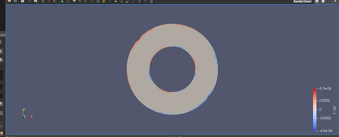
In fact, if I enforce the BC as @Stein suggested by replacing - n[i] * (v.dx( i )) * nu_w * ds with - n[i] * gradv_expression * nu_w * ds and plot the ‘residual’ of the solution \nabla^2 w - f by setting a different color scale, it significantly differs from zero also in the bulk, where it should not:

On the other hand, if I enforce the Dirichlet BCs for w by setting

w_profile = Expression( '8 * (sin( 2 * x[0] ) - sin( 2 * x[1] ))', L=L, h=h, element=Q.sub( 2 ).ufl_element() )
bc_w = DirichletBC( Q.sub( 2 ), w_profile, boundary )
bcs = [bc_u, bc_v, bc_w]

the ‘residual’ looks fine

So there is something wrong here. Given that this is issue somewhat departs from the original question of this post, where I saw that the residual took huge values, and which have been fixed by this reply, I will open a new post where I clearly re-formulat the question about this latter point.