Solve unsteady NS

[elabb]

Hello,
I am having trouble to get the solution of incompressible Navier-Stokes DFG benchmark 2D-2 (RE100, periodic) - Featflow (tu-dortmund.de) for different time steps.
I edit the code in the Dokken’s FEniCSx tutorial for the flow past a cylinder (Test problem 2: Flow past a cylinder (DFG 2D-3 benchmark) — FEniCSx tutorial ), but did not get the desire result.
the complete code is:

import gmsh
import os
import numpy as np
import matplotlib.pyplot as plt
import tqdm.autonotebook
import matplotlib as mpl

from mpi4py import MPI
from petsc4py import PETSc

from dolfinx.cpp.mesh import to_type, cell_entity_type
from dolfinx.fem import (Constant, Function, FunctionSpace,
                         assemble_scalar, dirichletbc, form, locate_dofs_topological, set_bc)
from dolfinx.fem.petsc import (apply_lifting, assemble_matrix, assemble_vector,
                               create_vector, create_matrix, set_bc)
from dolfinx.graph import adjacencylist
from dolfinx.geometry import bb_tree, compute_collisions_points, compute_colliding_cells
from dolfinx.io import (VTXWriter, distribute_entity_data, gmshio)
from dolfinx.mesh import create_mesh, meshtags_from_entities

from dolfinx import plot

from ufl import (FacetNormal, FiniteElement, Identity, Measure, TestFunction, TrialFunction, VectorElement,
                 as_vector, div, dot, ds, dx, inner, lhs, grad, nabla_grad, rhs, sym)

import dolfinx
import viskex

import matplotlib.tri as tri

mesh_comm = MPI.COMM_WORLD

############################################
#--------------- Mesh creation ------------#
############################################
model_rank = 0
gmsh.initialize()

L = 2.2
H = 0.41
c_x = c_y = 0.2
r = 0.05
gdim = 2

## Creation of the geometry entities (a cylinder within a rectangle)
if mesh_comm.rank == model_rank:
    rectangle = gmsh.model.occ.addRectangle(0, 0, 0, L, H, tag=1)
    obstacle = gmsh.model.occ.addDisk(c_x, c_y, 0, r, r)

## The next step is to substract the obstacle from the channel, such that we do not mesh the interior of the circle
if mesh_comm.rank == model_rank:
    fluid = gmsh.model.occ.cut([(gdim, rectangle)], [(gdim, obstacle)])
    gmsh.model.occ.synchronize()

## To get GMSH to mesh the fluid, we add a physical volume marker
fluid_marker = 1
if mesh_comm.rank == model_rank:
    volumes = gmsh.model.getEntities(dim=gdim)
    assert (len(volumes) == 1)
    gmsh.model.addPhysicalGroup(volumes[0][0], [volumes[0][1]], fluid_marker)
    gmsh.model.setPhysicalName(volumes[0][0], fluid_marker, "Fluid")

## To get GMSH to mesh the fluid, we add a physical volume marker
fluid_marker = 1
if mesh_comm.rank == model_rank:
    volumes = gmsh.model.getEntities(dim=gdim)
    assert (len(volumes) == 1)
    gmsh.model.addPhysicalGroup(volumes[0][0], [volumes[0][1]], fluid_marker)
    gmsh.model.setPhysicalName(volumes[0][0], fluid_marker, "Fluid")

#  variable mesh sizes to resolve the flow solution in the area of interest; close to the circular obstacle

# Create distance field from obstacle.
# Add threshold of mesh sizes based on the distance field
# LcMax -                  /--------
#                      /
# LcMin -o---------/
#        |         |       |
#       Point    DistMin DistMax
res_min = r / 3
if mesh_comm.rank == model_rank:
    distance_field = gmsh.model.mesh.field.add("Distance")
    gmsh.model.mesh.field.setNumbers(distance_field, "EdgesList", obstacle)
    threshold_field = gmsh.model.mesh.field.add("Threshold")
    gmsh.model.mesh.field.setNumber(threshold_field, "IField", distance_field)
    gmsh.model.mesh.field.setNumber(threshold_field, "LcMin", res_min)
    gmsh.model.mesh.field.setNumber(threshold_field, "LcMax", 0.25 * H)
    gmsh.model.mesh.field.setNumber(threshold_field, "DistMin", r)
    gmsh.model.mesh.field.setNumber(threshold_field, "DistMax", 2 * H)
    min_field = gmsh.model.mesh.field.add("Min")
    gmsh.model.mesh.field.setNumbers(min_field, "FieldsList", [threshold_field])
    gmsh.model.mesh.field.setAsBackgroundMesh(min_field)

### GENERATING THE MESH
## We are now ready to generate the mesh. However, we have to decide if our mesh should
## consist of triangles or quadrilaterals. Here we use second order quadrilateral elements.

if mesh_comm.rank == model_rank:
    gmsh.option.setNumber("Mesh.Algorithm", 8)
    gmsh.option.setNumber("Mesh.RecombinationAlgorithm", 2)
    gmsh.option.setNumber("Mesh.RecombineAll", 1)
    gmsh.option.setNumber("Mesh.SubdivisionAlgorithm", 1)
    gmsh.model.mesh.generate(gdim)
    gmsh.model.mesh.setOrder(2)
    gmsh.model.mesh.optimize("Netgen")

#=============== Loading mesh and boundary markers============================
## As we have generated the mesh, we now need to load the mesh and corresponding
## facet markers into DOLFINx. 
mesh, c, ft = gmshio.model_to_mesh(gmsh.model, mesh_comm, model_rank, gdim=gdim)
mesh.name = "Cylinder"
c.name = "Cell markers"
ft.name = "Facet markers"
# gmsh.finalize()
# mesh.topology.create_connectivity(mesh.topology.dim - 1, mesh.topology.dim)

# Physical and discretization parameters

t = 0
T = 8                      # Final time
dt =1 / 5                # Time step size
num_steps =int(T / dt)
k = Constant(mesh, PETSc.ScalarType(dt))
mu = Constant(mesh, PETSc.ScalarType(0.001))  # Dynamic viscosity
rho = Constant(mesh, PETSc.ScalarType(1))     # Density

#=================== Boundary conditions===========================

v_cg2 = VectorElement("Lagrange", mesh.ufl_cell(), 2)
s_cg1 = FiniteElement("Lagrange", mesh.ufl_cell(), 1)
V = FunctionSpace(mesh, v_cg2)
Q = FunctionSpace(mesh, s_cg1)

fdim = mesh.topology.dim - 1

# Define boundary conditions
U_0 = 0.3 # longitunal/lenghtwise velocity at coordinate (x,y)=(0,H/2)

# class InletVelocity():
#     def __init__(self, t):
#         self.t = t

#     def __call__(self, x):
#         values = np.zeros((gdim, x.shape[1]), dtype=PETSc.ScalarType)
#         # Umax=1.5
#         # values[0] = 4 * 1.5 * np.sin(self.t * np.pi / 8) * x[1] * (0.41 - x[1]) / (0.41**2)
#         values[0] = 4 * 1.5  * x[1] * (H - x[1]) / (H**2)
#         # values[0, :] = 0.3
#         return values
    
def u_in_eval(x: np.typing.NDArray[np.float64]) -> np.typing.NDArray[  # type: ignore[no-any-unimported]
        PETSc.ScalarType]:
    """Return the flat velocity profile at the inlet."""
    values = np.zeros((2, x.shape[1]))
    values[0] = 4 * U_0 * x[1] * (H - x[1])/(H**2)
    # values[0, :] = 1.5
    return values

# Inlet
u_inlet = Function(V)
# inlet_velocity = InletVelocity(t)
u_inlet.interpolate(u_in_eval)
bcu_inflow = dirichletbc(u_inlet, locate_dofs_topological(V, fdim, ft.find(inlet_marker)))
# Walls
u_nonslip = np.array((0,) * mesh.geometry.dim, dtype=PETSc.ScalarType)
bcu_walls = dirichletbc(u_nonslip, locate_dofs_topological(V, fdim, ft.find(wall_marker)), V)
# Obstacle
bcu_obstacle = dirichletbc(u_nonslip, locate_dofs_topological(V, fdim, ft.find(obstacle_marker)), V)
bcu = [bcu_inflow, bcu_obstacle, bcu_walls]
# Outlet
bcp_outlet = dirichletbc(PETSc.ScalarType(0), locate_dofs_topological(Q, fdim, ft.find(outlet_marker)), Q)
bcp = [bcp_outlet]

#============== Variational form============================
u = TrialFunction(V)
v = TestFunction(V)
u_ = Function(V)
u_.name = "u"
u_s = Function(V)
u_n = Function(V)  #uold
u_n1 = Function(V)
p = TrialFunction(Q)
q = TestFunction(Q)
p_ = Function(Q)
p_.name = "p"
phi = Function(Q)

# variational formulation for the first step
f = Constant(mesh, PETSc.ScalarType((0, 0)))
F1 = rho / k * dot(u - u_n, v) * dx
F1 += inner(dot(1.5 * u_n - 0.5 * u_n1, 0.5 * nabla_grad(u + u_n)), v) * dx
F1 += 0.5 * mu * inner(grad(u + u_n), grad(v)) * dx - dot(p_, div(v)) * dx
F1 += dot(f, v) * dx
a1 = form(lhs(F1))
L1 = form(rhs(F1))
A1 = create_matrix(a1)
b1 = create_vector(L1)

#  the second step
a2 = form(dot(grad(p), grad(q)) * dx)
L2 = form(-rho / k * dot(div(u_s), q) * dx)
A2 = assemble_matrix(a2, bcs=bcp)
A2.assemble()
b2 = create_vector(L2)

# create the last step
a3 = form(rho * dot(u, v) * dx)
L3 = form(rho * dot(u_s, v) * dx - k * dot(nabla_grad(phi), v) * dx)
A3 = assemble_matrix(a3)
A3.assemble()
b3 = create_vector(L3)

# Solver for step 1
solver1 = PETSc.KSP().create(mesh.comm)
solver1.setOperators(A1)
solver1.setType(PETSc.KSP.Type.BCGS)
pc1 = solver1.getPC()
pc1.setType(PETSc.PC.Type.JACOBI)

# Solver for step 2
solver2 = PETSc.KSP().create(mesh.comm)
solver2.setOperators(A2)
solver2.setType(PETSc.KSP.Type.MINRES)
pc2 = solver2.getPC()
pc2.setType(PETSc.PC.Type.HYPRE)
pc2.setHYPREType("boomeramg")

# Solver for step 3
solver3 = PETSc.KSP().create(mesh.comm)
solver3.setOperators(A3)
solver3.setType(PETSc.KSP.Type.CG)
pc3 = solver3.getPC()
pc3.setType(PETSc.PC.Type.SOR)

#============ Verification of the implementation compute known physical quantities==============
n = -FacetNormal(mesh)  # Normal pointing out of obstacle
dObs = Measure("ds", domain=mesh, subdomain_data=ft, subdomain_id=obstacle_marker)
u_t = inner(as_vector((n[1], -n[0])), u_)
drag = form(2 / 0.1 * (mu / rho * inner(grad(u_t), n) * n[1] - p_ * n[0]) * dObs)
lift = form(-2 / 0.1 * (mu / rho * inner(grad(u_t), n) * n[0] + p_ * n[1]) * dObs)
if mesh.comm.rank == 0:
    C_D = np.zeros(num_steps, dtype=PETSc.ScalarType)
    C_L = np.zeros(num_steps, dtype=PETSc.ScalarType)
    t_u = np.zeros(num_steps, dtype=np.float64)
    t_p = np.zeros(num_steps, dtype=np.float64)

tree = bb_tree(mesh, mesh.geometry.dim)
points = np.array([[0.15, 0.2, 0], [0.25, 0.2, 0]])
cell_candidates = compute_collisions_points(tree, points)
colliding_cells = compute_colliding_cells(mesh, cell_candidates, points)
front_cells = colliding_cells.links(0)
back_cells = colliding_cells.links(1)
if mesh.comm.rank == 0:
    p_diff = np.zeros(num_steps, dtype=PETSc.ScalarType)

from dolfinx import geometry
pointsd = mesh.geometry.x

cells = []
points_on_proc = []
# Find cells whose bounding-box collide with the the points
cell_candidatesd = compute_collisions_points(tree, pointsd)
# Choose one of the cells that contains the point
colliding_cellsd = compute_colliding_cells(mesh, cell_candidatesd, pointsd)
for i, point in enumerate(pointsd):
    if len(colliding_cellsd.links(i)) > 0:
        points_on_proc.append(point)
        cells.append(colliding_cellsd.links(i)[0])

points_on_proc = np.array(points_on_proc, dtype=np.float64)

u_values =np.zeros((num_steps,points_on_proc.shape[0]))
v_values = np.zeros((num_steps,points_on_proc.shape[0]))
p_values = np.zeros((num_steps,points_on_proc.shape[0]))
times = np.zeros((num_steps,1))
# V0, dofs = V.sub(0).collapse()
# coords = V0.tabulate_dof_coordinates()[:, 0:2]#coords
# sort_coords = np.argsort(coords)


# Solving the time-dependent problem
from pathlib import Path
folder = Path("results")
folder.mkdir(exist_ok=True, parents=True)
vtx_u = VTXWriter(mesh.comm, "dfg2D-3-u.bp", [u_], engine="BP4")
vtx_p = VTXWriter(mesh.comm, "dfg2D-3-p.bp", [p_], engine="BP4")
vtx_u.write(t)
vtx_p.write(t)
progress = tqdm.autonotebook.tqdm(desc="Solving PDE", total=num_steps)
for i in range(num_steps):

    progress.update(1)
    # Update current time step
    t += dt
    # Update inlet velocity
    # inlet_velocity.t = t
    # u_inlet.interpolate(inlet_velocity)
    
    # Step 1: Tentative velocity step
    A1.zeroEntries()
    assemble_matrix(A1, a1, bcs=bcu)
    A1.assemble()
    with b1.localForm() as loc:
        loc.set(0)
    assemble_vector(b1, L1)
    apply_lifting(b1, [a1], [bcu])
    b1.ghostUpdate(addv=PETSc.InsertMode.ADD_VALUES, mode=PETSc.ScatterMode.REVERSE)
    set_bc(b1, bcu)
    solver1.solve(b1, u_s.vector)
    u_s.x.scatter_forward()

    # Step 2: Pressure corrrection step
    with b2.localForm() as loc:
        loc.set(0)
    assemble_vector(b2, L2)
    apply_lifting(b2, [a2], [bcp])
    b2.ghostUpdate(addv=PETSc.InsertMode.ADD_VALUES, mode=PETSc.ScatterMode.REVERSE)
    set_bc(b2, bcp)
    solver2.solve(b2, phi.vector)
    phi.x.scatter_forward()

    p_.vector.axpy(1, phi.vector)
    p_.x.scatter_forward()

    # Step 3: Velocity correction step
    with b3.localForm() as loc:
        loc.set(0)
    assemble_vector(b3, L3)
    b3.ghostUpdate(addv=PETSc.InsertMode.ADD_VALUES, mode=PETSc.ScatterMode.REVERSE)
    solver3.solve(b3, u_.vector)
    u_.x.scatter_forward()

    # Write solutions to file
    vtx_u.write(t)
    vtx_p.write(t)

    times[i,0]=t
    # valuesU.append(u_.x.array[dofs][sort_coords])
    # valuesP.append(p_.x.array[dofs][sort_coords])
    uval=u_.eval(points_on_proc, cells)
    pval=p_.eval(points_on_proc, cells)
    u_values[i,:]= uval[:,0]
    v_values[i,:]=uval[:,1]
    p_values[i,:] = pval[:,0]

    # Update variable with solution form this time step
    with u_.vector.localForm() as loc_, u_n.vector.localForm() as loc_n, u_n1.vector.localForm() as loc_n1:
        loc_n.copy(loc_n1)
        loc_.copy(loc_n)
        
    
    # Compute physical quantities
    # For this to work in paralell, we gather contributions from all processors
    # to processor zero and sum the contributions.
    drag_coeff = mesh.comm.gather(assemble_scalar(drag), root=0)
    lift_coeff = mesh.comm.gather(assemble_scalar(lift), root=0)
    p_front = None
    if len(front_cells) > 0:
        p_front = p_.eval(points[0], front_cells[:1])
    p_front = mesh.comm.gather(p_front, root=0)
    p_back = None
    if len(back_cells) > 0:
        p_back = p_.eval(points[1], back_cells[:1])
    p_back = mesh.comm.gather(p_back, root=0)
    if mesh.comm.rank == 0:
        t_u[i] = t
        t_p[i] = t - dt / 2
        C_D[i] = sum(drag_coeff)
        C_L[i] = sum(lift_coeff)
        # Choose first pressure that is found from the different processors
        for pressure in p_front:
            if pressure is not None:
                p_diff[i] = pressure[0]
                break
        for pressure in p_back:
            if pressure is not None:
                p_diff[i] -= pressure[0]
                break

vtx_u.close()
vtx_p.close()
t=0

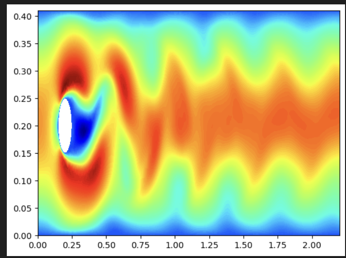
After I plot the solution values for different time frames the results are not logical.
the result of the velocity along x coordinates for last time frame is:

the actual result should be as:

Thanks.

[nate]

What’s the order of your time discretisation? I’ve seen similar results with backward Euler vs Crank Nicholson with the same problem before. I.e. the highly dissipative, first order accurate, backward Euler scheme gives almost laminar flow. Whereas the second order accurate Crank Nicholson method yields the Kármán vortex street as in your second picture.

[elabb]

the time dependent problem In the Dokken’s FEniCSx tutorial for the flow past a cylinder (Test problem 2: Flow past a cylinder (DFG 2D-3 benchmark) — FEniCSx tutorial) solved with respect to the inlet velocity and temporal discretization. So I believe that I should change the discretization to the second order backward difference or Crank-Nicholson. Could you say how I should edit my code to fullfil this task.
Thanks.

[dokken]

The code uses

As opposed to Pouseille flow, we will use a Crank-Nicolson discretization, and a semi-implicit Adams-Bashforth approximation.

Could you please point to what things you have changed from the tutorial, as it is quite tedious to go through them line by line to find the differences.

[elabb]

Hello,
for getting the solution values on all points for the mesh I used the following:

tree = bb_tree(mesh, mesh.geometry.dim)
pointsd = mesh.geometry.x

cells = []
points_on_proc = []
# Find cells whose bounding-box collide with the the points
cell_candidatesd = compute_collisions_points(tree, pointsd)
# Choose one of the cells that contains the point
colliding_cellsd = compute_colliding_cells(mesh, cell_candidatesd, pointsd)
for i, point in enumerate(pointsd):
    if len(colliding_cellsd.links(i)) > 0:
        points_on_proc.append(point)
        cells.append(colliding_cellsd.links(i)[0])

points_on_proc = np.array(points_on_proc, dtype=np.float64)

u_values =np.zeros((num_steps,points_on_proc.shape[0]))
v_values = np.zeros((num_steps,points_on_proc.shape[0]))
p_values = np.zeros((num_steps,points_on_proc.shape[0]))
times = np.zeros((num_steps,1))

in the for loop for updating the solution values I used:

    uval=u_.eval(points_on_proc, cells)
    pval=p_.eval(points_on_proc, cells)
    u_values[i,:]= uval[:,0]
    v_values[i,:]=uval[:,1]
    p_values[i,:] = pval[:,0]

but the result of my figure did not match with the correct solution and for all times my result show laminar solution.
I do not know what the reason is for such behavior.
Thanks

[dokken]

Wait? So you haven’t changed anything but the plotting in my script? Have you looked at the files outputted

vtx_u = VTXWriter(mesh.comm, "dfg2D-3-u.bp", [u_], engine="BP4")
vtx_p = VTXWriter(mesh.comm, "dfg2D-3-p.bp", [p_], engine="BP4")

in Paraview?

[elabb]

I also changed the U-inlet function as:

def u_in_eval(x: np.typing.NDArray[np.float64]) -> np.typing.NDArray[  # type: ignore[no-any-unimported]
        PETSc.ScalarType]:
    """Return the flat velocity profile at the inlet."""
    values = np.zeros((2, x.shape[1]))
    values[0] = 4 * U_0 * x[1] * (H - x[1])/(H**2)
    # values[0, :] = 1.5
    return values

the output of the last time frame for u in Paraview:

p output for the last timeframe in Paraview:

[dokken]

I cannot reproduce the latter plot that you have with the suggested modifications. You have also failed to rescale the veolcity at the last time step.
Comparing with: https://wwwold.mathematik.tu-dortmund.de/~featflow/en/benchmarks/cfdbenchmarking/flow/dfg_benchmark2_re100.html
you are using a way lower magnitude than them (0.3 vs 1.5).
If you run the code with a 1.5 magnitude on U_0, you get:

which at least from a visual point of view looks similar:

# ---
# jupyter:
#   jupytext:
#     formats: ipynb,py:light
#     text_representation:
#       extension: .py
#       format_name: light
#       format_version: '1.5'
#       jupytext_version: 1.14.7
#   kernelspec:
#     display_name: Python 3 (ipykernel)
#     language: python
#     name: python3
# ---

# # Test problem 2: Flow past a cylinder (DFG 2D-3 benchmark)
# Author: Jørgen S. Dokken
#
# In this section, we will turn our attention to a slightly more challenging problem: flow past a cylinder. The geometry and parameters are taken from the [DFG 2D-3 benchmark](https://www.featflow.de/en/benchmarks/cfdbenchmarking/flow/dfg_benchmark3_re100.html) in FeatFlow.
#
# To be able to solve this problem efficiently and ensure numerical stability, we will substitute our first order backward difference scheme with a Crank-Nicholson discretization in time, and a semi-implicit Adams-Bashforth approximation of the non-linear term.
#
# ```{admonition} Computationally demanding demo
# This demo is computationally demanding, with a run-time up to 15 minutes, as it is using parameters from the DFG 2D-3 benchmark, which consists of 12800 time steps. It is adviced to download this demo and  not run it in a browser. This runtime of the demo can be increased by using 2 or 3 mpi processes.
# ```
#
# The computational geometry we would like to use is
# ![Fluid channel with a circular obstacle](turek.png)
#
# The kinematic velocity is given by $\nu=0.001=\frac{\mu}{\rho}$ and the inflow velocity profile is specified as
#
# $$
#     u(x,y,t) = \left( \frac{4Uy(0.41-y)}{0.41^2}, 0 \right)
# $$
# $$
#     U=U(t) = 1.5\sin(\pi t/8)
# $$
#
# which has a maximum magnitude of $1.5$ at $y=0.41/2$. We do not use any scaling for this problem since all exact parameters are known.
# ## Mesh generation
# As in the [Deflection of a membrane](./../chapter1/membrane_code.ipynb) we use GMSH to generate the mesh. We fist create the rectangle and obstacle.

# +
import gmsh
import os
import numpy as np
import matplotlib.pyplot as plt
import tqdm.autonotebook

from mpi4py import MPI
from petsc4py import PETSc

from dolfinx.cpp.mesh import to_type, cell_entity_type
from dolfinx.fem import (Constant, Function, FunctionSpace,
                         assemble_scalar, dirichletbc, form, locate_dofs_topological, set_bc)
from dolfinx.fem.petsc import (apply_lifting, assemble_matrix, assemble_vector,
                               create_vector, create_matrix, set_bc)
from dolfinx.graph import adjacencylist
from dolfinx.geometry import bb_tree, compute_collisions_points, compute_colliding_cells
from dolfinx.io import (VTXWriter, distribute_entity_data, gmshio)
from dolfinx.mesh import create_mesh, meshtags_from_entities

from ufl import (FacetNormal, FiniteElement, Identity, Measure, TestFunction, TrialFunction, VectorElement,
                 as_vector, div, dot, ds, dx, inner, lhs, grad, nabla_grad, rhs, sym)

gmsh.initialize()

L = 2.2
H = 0.41
c_x = c_y = 0.2
r = 0.05
gdim = 2
mesh_comm = MPI.COMM_WORLD
model_rank = 0
if mesh_comm.rank == model_rank:
    rectangle = gmsh.model.occ.addRectangle(0, 0, 0, L, H, tag=1)
    obstacle = gmsh.model.occ.addDisk(c_x, c_y, 0, r, r)
# -

# The next step is to subtract the obstacle from the channel, such that we do not mesh the interior of the circle.

if mesh_comm.rank == model_rank:
    fluid = gmsh.model.occ.cut([(gdim, rectangle)], [(gdim, obstacle)])
    gmsh.model.occ.synchronize()

# To get GMSH to mesh the fluid, we add a physical volume marker

fluid_marker = 1
if mesh_comm.rank == model_rank:
    volumes = gmsh.model.getEntities(dim=gdim)
    assert (len(volumes) == 1)
    gmsh.model.addPhysicalGroup(volumes[0][0], [volumes[0][1]], fluid_marker)
    gmsh.model.setPhysicalName(volumes[0][0], fluid_marker, "Fluid")

# To tag the different surfaces of the mesh, we tag the inflow (left hand side) with marker 2, the outflow (right hand side) with marker 3 and the fluid walls with 4 and obstacle with 5. We will do this by compute the center of mass for each geometrical entitiy.

inlet_marker, outlet_marker, wall_marker, obstacle_marker = 2, 3, 4, 5
inflow, outflow, walls, obstacle = [], [], [], []
if mesh_comm.rank == model_rank:
    boundaries = gmsh.model.getBoundary(volumes, oriented=False)
    for boundary in boundaries:
        center_of_mass = gmsh.model.occ.getCenterOfMass(boundary[0], boundary[1])
        if np.allclose(center_of_mass, [0, H / 2, 0]):
            inflow.append(boundary[1])
        elif np.allclose(center_of_mass, [L, H / 2, 0]):
            outflow.append(boundary[1])
        elif np.allclose(center_of_mass, [L / 2, H, 0]) or np.allclose(center_of_mass, [L / 2, 0, 0]):
            walls.append(boundary[1])
        else:
            obstacle.append(boundary[1])
    gmsh.model.addPhysicalGroup(1, walls, wall_marker)
    gmsh.model.setPhysicalName(1, wall_marker, "Walls")
    gmsh.model.addPhysicalGroup(1, inflow, inlet_marker)
    gmsh.model.setPhysicalName(1, inlet_marker, "Inlet")
    gmsh.model.addPhysicalGroup(1, outflow, outlet_marker)
    gmsh.model.setPhysicalName(1, outlet_marker, "Outlet")
    gmsh.model.addPhysicalGroup(1, obstacle, obstacle_marker)
    gmsh.model.setPhysicalName(1, obstacle_marker, "Obstacle")

# In our previous meshes, we have used uniform mesh sizes. In this example, we will have variable mesh sizes to resolve the flow solution in  the area of interest; close to the circular obstacle. To do this, we use GMSH Fields.

# Create distance field from obstacle.
# Add threshold of mesh sizes based on the distance field
# LcMax -                  /--------
#                      /
# LcMin -o---------/
#        |         |       |
#       Point    DistMin DistMax
res_min = r / 3
if mesh_comm.rank == model_rank:
    distance_field = gmsh.model.mesh.field.add("Distance")
    gmsh.model.mesh.field.setNumbers(distance_field, "EdgesList", obstacle)
    threshold_field = gmsh.model.mesh.field.add("Threshold")
    gmsh.model.mesh.field.setNumber(threshold_field, "IField", distance_field)
    gmsh.model.mesh.field.setNumber(threshold_field, "LcMin", res_min)
    gmsh.model.mesh.field.setNumber(threshold_field, "LcMax", 0.25 * H)
    gmsh.model.mesh.field.setNumber(threshold_field, "DistMin", r)
    gmsh.model.mesh.field.setNumber(threshold_field, "DistMax", 2 * H)
    min_field = gmsh.model.mesh.field.add("Min")
    gmsh.model.mesh.field.setNumbers(min_field, "FieldsList", [threshold_field])
    gmsh.model.mesh.field.setAsBackgroundMesh(min_field)

# ## Generating the mesh
# We are now ready to generate the mesh. However, we have to decide if our mesh should consist of triangles or quadrilaterals. In this demo, to match the DFG 2D-3 benchmark, we use second order quadrilateral elements.

if mesh_comm.rank == model_rank:
    gmsh.option.setNumber("Mesh.Algorithm", 8)
    gmsh.option.setNumber("Mesh.RecombinationAlgorithm", 2)
    gmsh.option.setNumber("Mesh.RecombineAll", 1)
    gmsh.option.setNumber("Mesh.SubdivisionAlgorithm", 1)
    gmsh.model.mesh.generate(gdim)
    gmsh.model.mesh.setOrder(2)
    gmsh.model.mesh.optimize("Netgen")

# ## Loading mesh and boundary markers
# As we have generated the mesh, we now need to load the mesh and corresponding facet markers into DOLFINx.
# To load the mesh, we follow the same structure as in  [Deflection of a membrane](./../chapter1/membrane_code.ipynb), with the difference being that we will load in facet markers as well. To learn more about the specifics of the function below, see [A GMSH tutorial for DOLFINx](https://jsdokken.com/src/tutorial_gmsh.html).

mesh, _, ft = gmshio.model_to_mesh(gmsh.model, mesh_comm, model_rank, gdim=gdim)
ft.name = "Facet markers"

# ## Physical and discretization parameters
# Following the DGF-2 benchmark, we define our problem specific parameters

t = 0
T = 8                       # Final time
dt = 1 / 1600                 # Time step size
num_steps = int(T / dt)
k = Constant(mesh, PETSc.ScalarType(dt))
mu = Constant(mesh, PETSc.ScalarType(0.001))  # Dynamic viscosity
rho = Constant(mesh, PETSc.ScalarType(1))     # Density

# ```{admonition} Reduced end-time of problem
# In the current demo, we have reduced the run time to one second to make it easier to illustrate the concepts of the benchmark. By increasing the end-time `T` to 8, the runtime in a notebook is approximately 25 minutes. If you convert the notebook to a python file and use `mpirun`, you can reduce the runtime of the problem.
# ```
#
# ## Boundary conditions
# As we have created the mesh and relevant mesh tags, we can now specify the function spaces `V` and `Q` along with the boundary conditions. As the `ft` contains markers for facets, we use this class to find the facets for the inlet and walls.

# +
v_cg2 = VectorElement("Lagrange", mesh.ufl_cell(), 2)
s_cg1 = FiniteElement("Lagrange", mesh.ufl_cell(), 1)
V = FunctionSpace(mesh, v_cg2)
Q = FunctionSpace(mesh, s_cg1)

fdim = mesh.topology.dim - 1

# Define boundary conditions


class InletVelocity():
    def __init__(self, t):
        self.t = t

    def __call__(self, x):
        U_0 = 1.5
        values = np.zeros((gdim, x.shape[1]), dtype=PETSc.ScalarType)
        #values[0] = 4 * 1.5 * np.sin(self.t * np.pi / 8) * x[1] * (0.41 - x[1]) / (0.41**2)
        values[0] = 4 * U_0 * x[1] * (H - x[1])/(H**2)
        return values


# Inlet
u_inlet = Function(V)
inlet_velocity = InletVelocity(t)
u_inlet.interpolate(inlet_velocity)
bcu_inflow = dirichletbc(u_inlet, locate_dofs_topological(V, fdim, ft.find(inlet_marker)))
# Walls
u_nonslip = np.array((0,) * mesh.geometry.dim, dtype=PETSc.ScalarType)
bcu_walls = dirichletbc(u_nonslip, locate_dofs_topological(V, fdim, ft.find(wall_marker)), V)
# Obstacle
bcu_obstacle = dirichletbc(u_nonslip, locate_dofs_topological(V, fdim, ft.find(obstacle_marker)), V)
bcu = [bcu_inflow, bcu_obstacle, bcu_walls]
# Outlet
bcp_outlet = dirichletbc(PETSc.ScalarType(0), locate_dofs_topological(Q, fdim, ft.find(outlet_marker)), Q)
bcp = [bcp_outlet]
# -

# ## Variational form
# As opposed to [Pouseille flow](./ns_code1.ipynb), we will use a Crank-Nicolson discretization, and an semi-implicit Adams-Bashforth approximation.
# The first step can be written as
#
# $$
# \rho\left(\frac{u^*- u^n}{\delta t} + \left(\frac{3}{2}u^{n} - \frac{1}{2} u^{n-1}\right)\cdot \frac{1}{2}\nabla (u^*+u^n) \right) - \frac{1}{2}\mu \Delta( u^*+ u^n )+ \nabla p^{n-1/2} = f^{n+\frac{1}{2}} \qquad \text{ in } \Omega
# $$
#
# $$
# u^{*}=g(\cdot, t^{n+1}) \qquad \text{ on } \partial \Omega_{D}
# $$
#
# $$
# \frac{1}{2}\nu \nabla (u^*+u^n) \cdot n = p^{n-\frac{1}{2}} \qquad \text{ on } \partial \Omega_{N}
# $$
# where we have used the two previous time steps in the temporal derivative for the velocity, and compute the pressure staggered in time, at the time between the previous and current solution. The second step becomes
# $$
# \nabla \phi = -\frac{\rho}{\delta t} \nabla \cdot u^* \qquad\text{in } \Omega,
# $$
#
# $$
# \nabla \phi \cdot n = 0 \qquad \text{on } \partial \Omega_D,
# $$
#
# $$
# \phi = 0 \qquad\text{on } \partial\Omega_N
# $$
#
# where $p^{n+\frac{1}{2}}=p^{n-\frac{1}{2}} + \phi$.
# Finally, the third step is
#
# $$
# \rho (u^{n+1}-u^{*}) = -\delta t \phi.
# $$
#
# We start by defining all the variables used in the variational formulations.

u = TrialFunction(V)
v = TestFunction(V)
u_ = Function(V)
u_.name = "u"
u_s = Function(V)
u_n = Function(V)
u_n1 = Function(V)
p = TrialFunction(Q)
q = TestFunction(Q)
p_ = Function(Q)
p_.name = "p"
phi = Function(Q)

# Next, we define the variational formulation for the first step, where we have integrated the diffusion term, as well as the pressure term by parts.

f = Constant(mesh, PETSc.ScalarType((0, 0)))
F1 = rho / k * dot(u - u_n, v) * dx
F1 += inner(dot(1.5 * u_n - 0.5 * u_n1, 0.5 * nabla_grad(u + u_n)), v) * dx
F1 += 0.5 * mu * inner(grad(u + u_n), grad(v)) * dx - dot(p_, div(v)) * dx
F1 += dot(f, v) * dx
a1 = form(lhs(F1))
L1 = form(rhs(F1))
A1 = create_matrix(a1)
b1 = create_vector(L1)

# Next we define the second step

a2 = form(dot(grad(p), grad(q)) * dx)
L2 = form(-rho / k * dot(div(u_s), q) * dx)
A2 = assemble_matrix(a2, bcs=bcp)
A2.assemble()
b2 = create_vector(L2)

# We finally create the last step

a3 = form(rho * dot(u, v) * dx)
L3 = form(rho * dot(u_s, v) * dx - k * dot(nabla_grad(phi), v) * dx)
A3 = assemble_matrix(a3)
A3.assemble()
b3 = create_vector(L3)

# As in the previous tutorials, we use PETSc as a linear algebra backend.

# +
# Solver for step 1
solver1 = PETSc.KSP().create(mesh.comm)
solver1.setOperators(A1)
solver1.setType(PETSc.KSP.Type.BCGS)
pc1 = solver1.getPC()
pc1.setType(PETSc.PC.Type.JACOBI)

# Solver for step 2
solver2 = PETSc.KSP().create(mesh.comm)
solver2.setOperators(A2)
solver2.setType(PETSc.KSP.Type.MINRES)
pc2 = solver2.getPC()
pc2.setType(PETSc.PC.Type.HYPRE)
pc2.setHYPREType("boomeramg")

# Solver for step 3
solver3 = PETSc.KSP().create(mesh.comm)
solver3.setOperators(A3)
solver3.setType(PETSc.KSP.Type.CG)
pc3 = solver3.getPC()
pc3.setType(PETSc.PC.Type.SOR)
# -

# ## Verification of the implementation compute known physical quantities
# As a further verification of our implementation, we compute the drag and lift coefficients over the obstacle, defined as
#
# $$
#     C_{\text{D}}(u,p,t,\partial\Omega_S) = \frac{2}{\rho L U_{mean}^2}\int_{\partial\Omega_S}\rho \nu n \cdot \nabla u_{t_S}(t)n_y -p(t)n_x~\mathrm{d} s,
# $$
# $$
#     C_{\text{L}}(u,p,t,\partial\Omega_S) = -\frac{2}{\rho L U_{mean}^2}\int_{\partial\Omega_S}\rho \nu n \cdot \nabla u_{t_S}(t)n_x + p(t)n_y~\mathrm{d} s,
# $$
#
# where $u_{t_S}$ is the tangential velocity component at the interface of the obstacle $\partial\Omega_S$, defined as $u_{t_S}=u\cdot (n_y,-n_x)$, $U_{mean}=1$ the average inflow velocity, and $L$ the length of the channel. We use `UFL` to create the relevant integrals, and assemble them at each time step.

n = -FacetNormal(mesh)  # Normal pointing out of obstacle
dObs = Measure("ds", domain=mesh, subdomain_data=ft, subdomain_id=obstacle_marker)
u_t = inner(as_vector((n[1], -n[0])), u_)
drag = form(2 / 0.1 * (mu / rho * inner(grad(u_t), n) * n[1] - p_ * n[0]) * dObs)
lift = form(-2 / 0.1 * (mu / rho * inner(grad(u_t), n) * n[0] + p_ * n[1]) * dObs)
if mesh.comm.rank == 0:
    C_D = np.zeros(num_steps, dtype=PETSc.ScalarType)
    C_L = np.zeros(num_steps, dtype=PETSc.ScalarType)
    t_u = np.zeros(num_steps, dtype=np.float64)
    t_p = np.zeros(num_steps, dtype=np.float64)

# We will also evaluate the pressure at two points, on in front of the obstacle, $(0.15, 0.2)$, and one behind the obstacle, $(0.25, 0.2)$. To do this, we have to find which cell is containing each of the points, so that we can create a linear combination of the local basis functions and coefficients.

tree = bb_tree(mesh, mesh.geometry.dim)
points = np.array([[0.15, 0.2, 0], [0.25, 0.2, 0]])
cell_candidates = compute_collisions_points(tree, points)
colliding_cells = compute_colliding_cells(mesh, cell_candidates, points)
front_cells = colliding_cells.links(0)
back_cells = colliding_cells.links(1)
if mesh.comm.rank == 0:
    p_diff = np.zeros(num_steps, dtype=PETSc.ScalarType)

# ## Solving the time-dependent problem
# ```{admonition} Stability of the Navier-Stokes equation
# Note that the current splitting scheme has to fullfil the a [Courant–Friedrichs–Lewy condition](https://en.wikipedia.org/wiki/Courant%E2%80%93Friedrichs%E2%80%93Lewy_condition). This limits the spatial discretization with respect to the inlet velocity and temporal discretization.
# Other temporal discretization schemes such as the second order backward difference discretization or Crank-Nicholson discretization with Adams-Bashforth linearization are better behaved than our simple backward difference scheme.
# ```
#
# As in the previous example, we create output files for the velocity and pressure and solve the time-dependent problem. As we are solving a time dependent problem with many time steps, we use the `tqdm`-package to visualize the progress. This package can be install with `pip3`.

from pathlib import Path
folder = Path("results")
folder.mkdir(exist_ok=True, parents=True)
vtx_u = VTXWriter(mesh.comm, "dfg2D-3-u.bp", [u_], engine="BP4")
vtx_p = VTXWriter(mesh.comm, "dfg2D-3-p.bp", [p_], engine="BP4")
vtx_u.write(t)
vtx_p.write(t)
progress = tqdm.autonotebook.tqdm(desc="Solving PDE", total=num_steps)
for i in range(num_steps):
    progress.update(1)
    # Update current time step
    t += dt
    # Update inlet velocity
    inlet_velocity.t = t
    u_inlet.interpolate(inlet_velocity)

    # Step 1: Tentative velocity step
    A1.zeroEntries()
    assemble_matrix(A1, a1, bcs=bcu)
    A1.assemble()
    with b1.localForm() as loc:
        loc.set(0)
    assemble_vector(b1, L1)
    apply_lifting(b1, [a1], [bcu])
    b1.ghostUpdate(addv=PETSc.InsertMode.ADD_VALUES, mode=PETSc.ScatterMode.REVERSE)
    set_bc(b1, bcu)
    solver1.solve(b1, u_s.vector)
    u_s.x.scatter_forward()

    # Step 2: Pressure corrrection step
    with b2.localForm() as loc:
        loc.set(0)
    assemble_vector(b2, L2)
    apply_lifting(b2, [a2], [bcp])
    b2.ghostUpdate(addv=PETSc.InsertMode.ADD_VALUES, mode=PETSc.ScatterMode.REVERSE)
    set_bc(b2, bcp)
    solver2.solve(b2, phi.vector)
    phi.x.scatter_forward()

    p_.vector.axpy(1, phi.vector)
    p_.x.scatter_forward()

    # Step 3: Velocity correction step
    with b3.localForm() as loc:
        loc.set(0)
    assemble_vector(b3, L3)
    b3.ghostUpdate(addv=PETSc.InsertMode.ADD_VALUES, mode=PETSc.ScatterMode.REVERSE)
    solver3.solve(b3, u_.vector)
    u_.x.scatter_forward()

    # Write solutions to file
    vtx_u.write(t)
    vtx_p.write(t)

    # Update variable with solution form this time step
    with u_.vector.localForm() as loc_, u_n.vector.localForm() as loc_n, u_n1.vector.localForm() as loc_n1:
        loc_n.copy(loc_n1)
        loc_.copy(loc_n)

    # Compute physical quantities
    # For this to work in paralell, we gather contributions from all processors
    # to processor zero and sum the contributions.
    drag_coeff = mesh.comm.gather(assemble_scalar(drag), root=0)
    lift_coeff = mesh.comm.gather(assemble_scalar(lift), root=0)
    p_front = None
    if len(front_cells) > 0:
        p_front = p_.eval(points[0], front_cells[:1])
    p_front = mesh.comm.gather(p_front, root=0)
    p_back = None
    if len(back_cells) > 0:
        p_back = p_.eval(points[1], back_cells[:1])
    p_back = mesh.comm.gather(p_back, root=0)
    if mesh.comm.rank == 0:
        t_u[i] = t
        t_p[i] = t - dt / 2
        C_D[i] = sum(drag_coeff)
        C_L[i] = sum(lift_coeff)
        # Choose first pressure that is found from the different processors
        for pressure in p_front:
            if pressure is not None:
                p_diff[i] = pressure[0]
                break
        for pressure in p_back:
            if pressure is not None:
                p_diff[i] -= pressure[0]
                break
vtx_u.close()
vtx_p.close()

[elabb]

Thanks I got this solution before, but I want to have only 40 time-steps. So when I choose dt as follow:

dt = 1 / 5                 # Time step size

I get the following results:

is there any way to have the correct solution for only 40 time-steps.
I think I should move to mixed-element with Newton solver.

[dokken]

You cannot reduce the time-step with that amount. You need to fullfil the CFL condition: Courant–Friedrichs–Lewy condition - Wikipedia
which means that you would need a coarser grid.

You would also have issues with starting from a zero initial guess, as you send in a better initial solution.

Please note that for further questions on the subject, it would be good if you include all the changes you did in a summary from the get-go.

[elabb]

Aha, that’s the reason.
Can you give me any hint or a sample code for a splitting scheme that would fulfill my desire? I mean solving the issue with lower time-steps.

[dokken]

Not sure there is a splitting scheme that can do that, you would have to investigate papers referenced on Splitting schemes — Oasisx and papers citing these.

Why do you want this very coarse time-step?

[elabb]

I need 40 time-steps data for ML algorithm and 12000 time-steps would increase the training time.
I also used the mixed-element for solving the issue with 40 time steps and using Crank-Nicholson but I got laminar results. the code is as follow:

up = Function(W)

u, p = split(up)

up_old = Function(W)
u_old, p_old = split(up_old)

(v, q) = TestFunctions(W)

F = ((1/dt)*dot(u - u_old, v)
  + (theta)*nu * inner(grad(u), grad(v))
  + (theta)*dot(dot(grad(u),u),v)
  + (1-theta)*nu * inner(grad(u_old), grad(v))
  + (1-theta)*dot(dot(grad(u_old),u_old),v)
  - p * div(v)
  - q * div(u)
    ) * dx

Newton solver:

problem = NonlinearProblem(F, up, bcu)
solver = NewtonSolver(MPI.COMM_WORLD, problem)

solver.rtol = 1e-6

ksp = solver.krylov_solver
opts = PETSc.Options()
option_prefix = ksp.getOptionsPrefix()
opts[f"{option_prefix}ksp_type"] = "preonly"
opts[f"{option_prefix}pc_type"] = "lu"
opts[f"{option_prefix}pc_factor_mat_solver_type"] = "mumps"
ksp.setFromOptions()

# Step in time
t = 0.0
up_old.x.array[:] = up.x.array
ii=0
while (t < T):
    ii += 1
    t += float(dt)
    r = solver.solve(up)
    print(f"Step {int(t/float(dt))}: num iterations: {r[0]}")
    up_old.x.array[:] = up.x.array

I do not know how to rescale the velocity for the Newtonsolver if needed.

[dokken]

You should try something in between 40 and 12800 time steps.
The run-time of the problem is a few minutes, so generating training data shouldn’t be that expensive.

[elabb]

Ok I could get the result by 40 time-steps when I increase the velocity in the mixed-element scheme.

for anyone who in need of the complete code of mixed element for unsteady navier-stokes problem :

# https://fenicsproject.discourse.group/t/incompressible-navier-stokes-with-particular-scheme-mixed-elements-fenicsx/10249
# https://wwwold.mathematik.tu-dortmund.de/~featflow/en/benchmarks/cfdbenchmarking/flow/dfg_benchmark2_re100.html
############################################
#--------------- Imports ------------------#
############################################
import dolfinx
import gmsh
import numpy as np
from mpi4py import MPI
from petsc4py import PETSc
from dolfinx.fem import (Constant, Function, dirichletbc)
from dolfinx.fem.petsc import  NonlinearProblem

from dolfinx.io import gmshio
from ufl import (TestFunctions, div,dx, dot, inner, grad, split)
from dolfinx.nls.petsc import NewtonSolver
import basix.ufl

mesh_comm = MPI.COMM_WORLD


############################################
#--------------- Mesh creation ------------#
############################################
model_rank = 0
gmsh.initialize()

# L = 3e-4
# H = 5e-5
# c_x , c_y = (5e-5, 25e-6)
# r = 25e-7
L = 2.2
H = 0.41
c_x = c_y = 0.2
r = 0.05
gdim = 2

## Creation of the geometry entities (a cylinder within a rectangle)
if mesh_comm.rank == model_rank:
    rectangle = gmsh.model.occ.addRectangle(0, 0, 0, L, H, tag=1)
    obstacle = gmsh.model.occ.addDisk(c_x, c_y, 0, r, r)

## The next step is to substract the obstacle from the channel, such that we do not mesh the interior of the circle
if mesh_comm.rank == model_rank:
    fluid = gmsh.model.occ.cut([(gdim, rectangle)], [(gdim, obstacle)])
    gmsh.model.occ.synchronize()


## To get GMSH to mesh the fluid, we add a physical volume marker
fluid_marker = 1
if mesh_comm.rank == model_rank:
    volumes = gmsh.model.getEntities(dim=gdim)
    assert (len(volumes) == 1)
    gmsh.model.addPhysicalGroup(volumes[0][0], [volumes[0][1]], fluid_marker)
    gmsh.model.setPhysicalName(volumes[0][0], fluid_marker, "Fluid")

## To tag the different surfaces of the mesh, we tag the inflow (left hand side) with marker 2, the outflow (right hand side)
## with marker 3 and the fluid walls with 4 and obstacle with 5. We will do this by computing the center of mass for each geometrical
## entity.

inlet_marker, outlet_marker, wall_marker, obstacle_marker = 2, 3, 4, 5
inflow, outflow, walls, obstacle = [], [], [], []
if mesh_comm.rank == model_rank:
    boundaries = gmsh.model.getBoundary(volumes, oriented=False)
    for boundary in boundaries:
        center_of_mass = gmsh.model.occ.getCenterOfMass(boundary[0], boundary[1])
        if np.allclose(center_of_mass, [0, H / 2, 0]):
            inflow.append(boundary[1])
        elif np.allclose(center_of_mass, [L, H / 2, 0]):
            outflow.append(boundary[1])
        elif np.allclose(center_of_mass, [L / 2, H, 0]) or np.allclose(center_of_mass, [L / 2, 0, 0]):
            walls.append(boundary[1])
        else:
            obstacle.append(boundary[1])
    gmsh.model.addPhysicalGroup(1, walls, wall_marker)
    gmsh.model.setPhysicalName(1, wall_marker, "Walls")
    gmsh.model.addPhysicalGroup(1, inflow, inlet_marker)
    gmsh.model.setPhysicalName(1, inlet_marker, "Inlet")
    gmsh.model.addPhysicalGroup(1, outflow, outlet_marker)
    gmsh.model.setPhysicalName(1, outlet_marker, "Outlet")
    gmsh.model.addPhysicalGroup(1, obstacle, obstacle_marker)
    gmsh.model.setPhysicalName(1, obstacle_marker, "Obstacle")


#  variable mesh sizes to resolve the flow solution in the area of interest; close to the circular obstacle

# Create distance field from obstacle.
# Add threshold of mesh sizes based on the distance field
# LcMax -                  /--------
#                      /
# LcMin -o---------/
#        |         |       |
#       Point    DistMin DistMax
res_min = r / 3
if mesh_comm.rank == model_rank:
    distance_field = gmsh.model.mesh.field.add("Distance")
    gmsh.model.mesh.field.setNumbers(distance_field, "EdgesList", obstacle)
    threshold_field = gmsh.model.mesh.field.add("Threshold")
    gmsh.model.mesh.field.setNumber(threshold_field, "IField", distance_field)
    gmsh.model.mesh.field.setNumber(threshold_field, "LcMin", res_min)
    gmsh.model.mesh.field.setNumber(threshold_field, "LcMax", 0.25 * H)
    gmsh.model.mesh.field.setNumber(threshold_field, "DistMin", r)
    gmsh.model.mesh.field.setNumber(threshold_field, "DistMax", 2 * H)
    min_field = gmsh.model.mesh.field.add("Min")
    gmsh.model.mesh.field.setNumbers(min_field, "FieldsList", [threshold_field])
    gmsh.model.mesh.field.setAsBackgroundMesh(min_field)


### GENERATING THE MESH
## We are now ready to generate the mesh. However, we have to decide if our mesh should
## consist of triangles or quadrilaterals. Here we use second order quadrilateral elements.

if mesh_comm.rank == model_rank:
    gmsh.option.setNumber("Mesh.Algorithm", 8)
    gmsh.option.setNumber("Mesh.RecombinationAlgorithm", 2)
    gmsh.option.setNumber("Mesh.RecombineAll", 1)
    gmsh.option.setNumber("Mesh.SubdivisionAlgorithm", 1)
    gmsh.model.mesh.generate(gdim)
    gmsh.model.mesh.setOrder(2)
    gmsh.model.mesh.optimize("Netgen")

#=============== Loading mesh and boundary markers============================
## As we have generated the mesh, we now need to load the mesh and corresponding
## facet markers into DOLFINx. See https://jsdokken.com/src/tutorial_gmsh.html for explanations
mesh, c, ft = gmshio.model_to_mesh(gmsh.model, mesh_comm, model_rank, gdim=gdim)
mesh.name = "Cylinder"
c.name = "Cell markers"
ft.name = "Facet markers"

############################################
#--- Parameters & boudnary conditions -----#
############################################
## We define our problem specific parameters
dt = Constant(mesh, PETSc.ScalarType(1/5))
nu = Constant(mesh, PETSc.ScalarType(0.001/1)) # nu = 1/Re
T = 8         # Final time
theta = 0.5  # time stepping family, e.g. theta=1 -> backward Euler, theta=0.5 -> Crank-Nicholson
relax = Constant(mesh, PETSc.ScalarType(1e-6)) # relaxation constant
U_0 = 1.5 # longitunal/lenghtwise velocity at coordinate (x,y)=(0,H/2)

# Inlet velocity profile
def u_in_eval(x: np.typing.NDArray[np.float64]) -> np.typing.NDArray[  # type: ignore[no-any-unimported]
        PETSc.ScalarType]:
    """Return the flat velocity profile at the inlet."""
    values = np.zeros((2, x.shape[1]))
    values[0] = 4 * U_0 * x[1] * (H - x[1])/(H**2)
    # values[0, :] = 1.5
    return values

def u_wall_eval(x: np.typing.NDArray[np.float64]) -> np.typing.NDArray[  # type: ignore[no-any-unimported]
        PETSc.ScalarType]:
    """Return the zero velocity at the wall."""
    return np.zeros((2, x.shape[1]))

## As we have created the mesh and relevant mesh tags, we can now specify the function
## spaces V aand Q along with the boundary conditions. As the ft contains markers for facets,
## we use this class to find the facets for the inlet and walls.
	
V_element = basix.ufl.element("Lagrange", mesh.basix_cell(), 2, shape=(mesh.geometry.dim, ))
Q_element = basix.ufl.element("Lagrange", mesh.basix_cell(), 1)

W_element = basix.ufl.mixed_element([V_element, Q_element])
W = dolfinx.fem.functionspace(mesh, W_element)

V, _ = W.sub(0).collapse()
Q, _ = W.sub(1).collapse()

fdim = mesh.topology.dim - 1

# DOLFIN_EPS = 0.000001

def Inflow(x):
    # return np.abs(x[0] - 0.) < DOLFIN_EPS
	return  np.isclose(x[0], 0)



def Walls(x):
	return np.logical_or(np.isclose(x[1], 0), np.isclose(x[1], H))


def Obstacle(x):
    return np.isclose(np.sqrt(x[0]**2 + x[1]**2), r)

# Inlet
u_inlet = Function(V)
u_inlet.interpolate(u_in_eval)
inflow_facets = dolfinx.mesh.locate_entities_boundary(mesh, fdim,
                                                      Inflow)
inflow_dofs = dolfinx.fem.locate_dofs_topological((W.sub(0), V), fdim,
                                                  ft.indices[ft.values == 2])
bcu_inflow = dolfinx.fem.dirichletbc(u_inlet, inflow_dofs, W.sub(0))

# Walls
u_nonslip = dolfinx.fem.Function(V)
u_nonslip.interpolate(u_wall_eval)
wall_facets = dolfinx.mesh.locate_entities_boundary(mesh, fdim,
                                                      Walls)
wall_dofs = dolfinx.fem.locate_dofs_topological((W.sub(0), V), fdim,
                                                  ft.indices[ft.values == 4])

bcu_walls = dolfinx.fem.dirichletbc(u_nonslip, wall_dofs, W.sub(0))

# Obstacle
Obstacle_facets = dolfinx.mesh.locate_entities_boundary(mesh,fdim,
                                                      Obstacle)
Obstacle_dofs = dolfinx.fem.locate_dofs_topological((W.sub(0), V),fdim,
                                                  ft.indices[ft.values == 5])
bcu_obstacle = dolfinx.fem.dirichletbc(u_nonslip, Obstacle_dofs, W.sub(0))

# grouping all boundary conditions involving the velocity u
bcu = [bcu_inflow, bcu_walls, bcu_obstacle]

# Outlet
p_outlet = PETSc.ScalarType(0)
outflow_dofs  = dolfinx.fem.locate_dofs_topological(Q, fdim,
                                                  ft.indices[ft.values == 3])
bcp_outlet = dirichletbc(p_outlet, outflow_dofs, W.sub(1))
# grouping all boundary conditions involving the pressure p
bcp = [bcp_outlet]



up = Function(W)

u, p = split(up)

up_old = Function(W)
u_old, p_old = split(up_old)

(v, q) = TestFunctions(W)


F = ((1/dt)*dot(u - u_old, v)
  + (theta)*nu * inner(grad(u), grad(v))
  + (theta)*dot(dot(grad(u),u),v)
  + (1-theta)*nu * inner(grad(u_old), grad(v))
  + (1-theta)*dot(dot(grad(u_old),u_old),v)
  - p * div(v)
  - q * div(u)
    ) * dx


problem = NonlinearProblem(F, up, bcu)
solver = NewtonSolver(MPI.COMM_WORLD, problem)

solver.rtol = 1e-6

ksp = solver.krylov_solver
opts = PETSc.Options()
option_prefix = ksp.getOptionsPrefix()
opts[f"{option_prefix}ksp_type"] = "preonly"
opts[f"{option_prefix}pc_type"] = "lu"
opts[f"{option_prefix}pc_factor_mat_solver_type"] = "mumps"
ksp.setFromOptions()


# Step in time
t = 0.0
# Get the sub-space for c and the corresponding dofs in the mixed space
# vector
V0, dofs = W.sub(0).collapse()
u = up.sub(0)
up_old.x.array[:] = up.x.array
ii=0
while (t < T):
    ii += 1
    t += float(dt)
    r = solver.solve(up)
    print(f"Step {int(t/float(dt))}: num iterations: {r[0]}")
    up_old.x.array[:] = up.x.array```

Thanks Dokken for your support.

[elabb]

one more question:
how I could implement the method in flow past a cylinder (Test problem 2: Flow past a cylinder (DFG 2D-3 benchmark) — FEniCSx tutorial ) for the stokes problem?

[dokken]

There are plenty of examples in the dolfinx docs on how to solve stokes equation. Please consult those docs.