Why does the basic 2D Stokes Equation fail for the to find a solution for an elliptical domain?

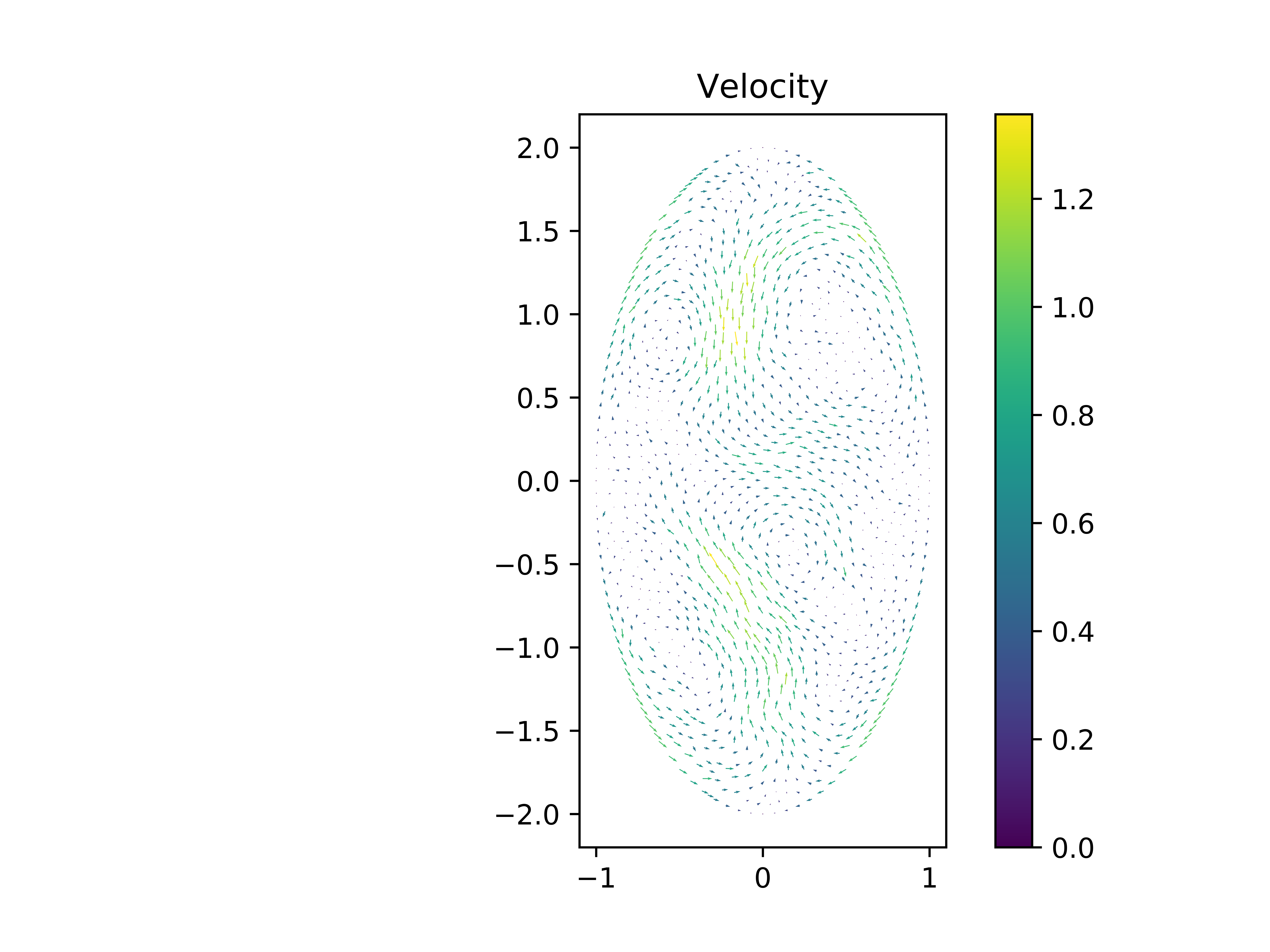
Resolved by fixing a typo. The code below should work.

I am using FEniCS 2018.1.0

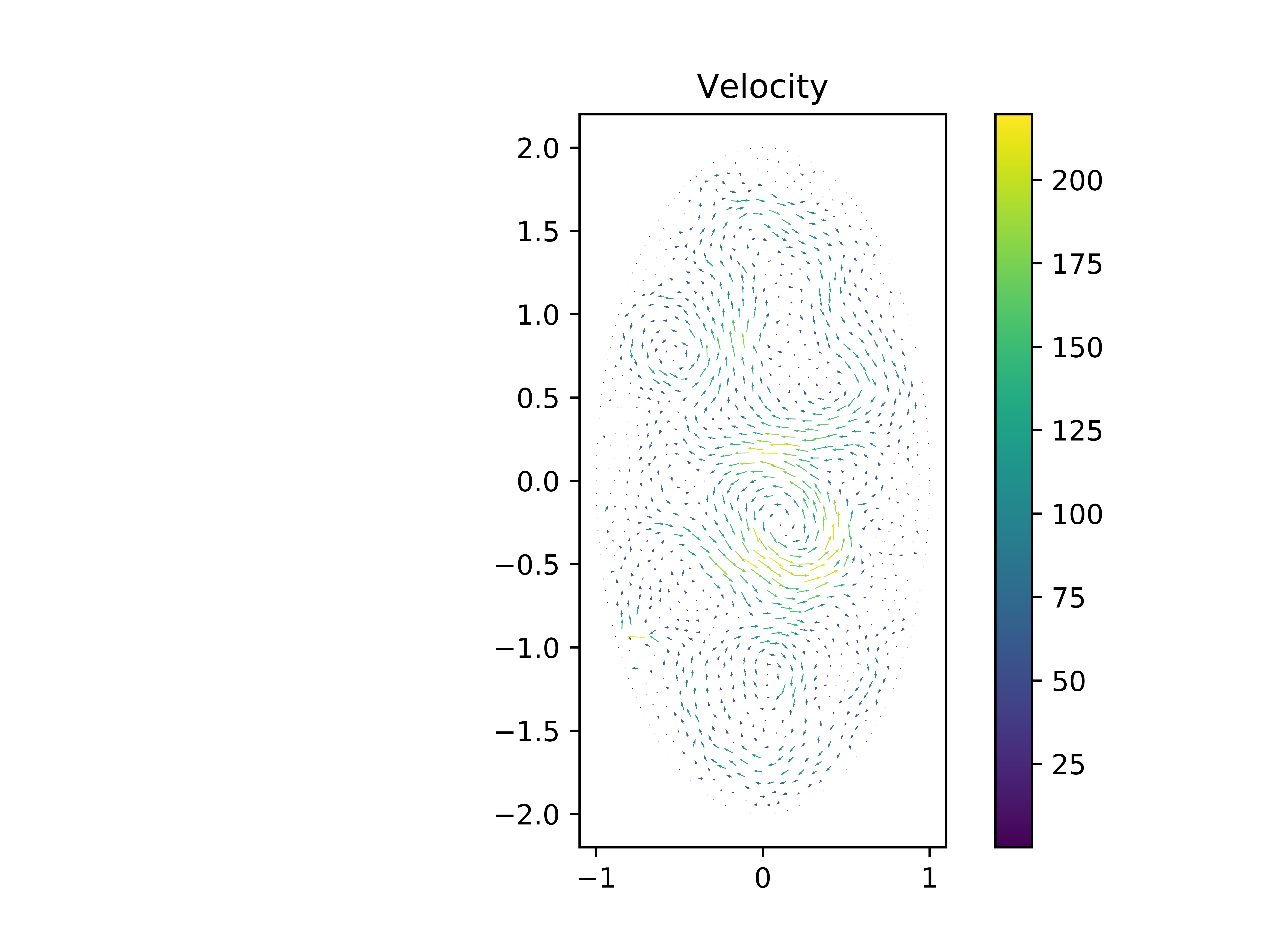
This might be because of the mesh, but the following code blows up for when b is not 1 and the boundary conditions have even harmonics. It is really bizzarre, since it works very well for odd harmonics. I am losing my mind figuring this out!

import matplotlib
matplotlib.use('Agg')
from matplotlib import ticker
import matplotlib.pyplot as plt
from dolfin import *
from mshr import *

def epsilon(u):
  return grad(u)+nabla_grad(u)

b=0.3
embryo = Ellipse(Point(0.0, 0.0), 1, b)
mesh = generate_mesh(embryo, 32)

# Define function spaces
P2 = VectorElement('CG', triangle, 5)
P1 = FiniteElement('CG', triangle, 3)
TH = MixedElement([P2, P1])
W = FunctionSpace(mesh, TH)
g = Constant(0.0)
mu = Constant(1.0)
force = Constant((0.0, 0.0))

# Specify Boundary Conditions
boundary = 'on_boundary'
flow_profile = ('-sin(atan2(x[1]/b,x[0]))*sin(nharmonic*atan2(x[1]/b,x[0]))','b*cos(atan2(x[1]/b,x[0]))*sin(nharmonic*atan2(x[1]/b,x[0]))')
bcu = DirichletBC(W.sub(0), Expression(flow_profile, degree=5, b=b, nharmonic=2), boundary)
bc = [bcu]

# Define trial and test functions
(u, p) = TrialFunctions(W)
(v, q) = TestFunctions(W)

a1 = inner( mu*epsilon(u)+p*Identity(2), nabla_grad(v))*dx + div(u)*q*dx
L1 = dot(force,v)*dx + g*q*dx
print('Preliminaries Done')

# Solve system
U = Function(W)
solve(a1==L1, U, bc)
print('Solving Done')

# Get sub-functions
u, p = U.split()

folder='./'
fig=plot(u, title='Velocity')
plt.colorbar(fig)
plt.savefig(folder+'vel.png', dpi=1000)
plt.close()
print('Plotting Done')

Hi!

I have tested your code under FEniCS 2018.2.0.dev0 with b=0.5 and b=2, and no errors were obtained. I recall you the following:

(1) A stable element for Stokes is given by, for instance, the Taylor-Hood element (P2,P1). There is no need of using (P5,P3), which is expensive when the mesh-size is small. See also the MINI-element.

(2) In general, the fluid pressure is unique up to an additive constant. To fix that, you can impose zero mean condition on the pressure. However, since your domain is changing with the value of b, you need to be careful with the manufactured data.

(3) The fluid velocity is not unique for Neumann conditions (on the whole boundary). You should, instead, require compatibility conditions and introduce a Lagrange multiplier. Other option is to use Dirichlet/mixed boundary conditions.

(4) For conforming finite elements like Tylor-Hood, local mass conservation (corresponding to the incompressibility of the fluid) is not expected. This can be achieved by using DG methods.

I hope this helps you!

Paulo

Hi Paolo,

Thanks for your answer! Could you share your plot with the solution for b=0.5 or b=2.0? While the solver does provide an answer, the answer is not reasonable. As a proof of the same, the variational problem is not solved.

  1. I tried using P2/P1 witha higher resultion as well, but I get the same answer. For my analysis, I need to take 4th order derivatives of the velocity, thus I would like to take P4/P2 elements at least. I also have non-linearities in the actual problem I am solving, and thus I get better solutions with higher-order elements.

  2. Since I only care about the gradient of the pressure, I don’t mind the additive constant unless it will cause my equation to fail.

  3. I am only using Dirichlet boundary conditions.

  4. My system requires mass-conservation. Though it may not be expected, I hope Taylor-Hood elements are not compatible with mass conservation (I can’t imagine why they would).

Thanks a lot once again for all your help!

Sorry for my delay in responding.

Hereby my results:

** b=0.5

** b=2

Hi Paolo, thanks for your response. Yes, I get the same plots, but as you can see, the flows are not physical. For one, the magnitude of flows inside is much much higher than the flows at the boundary, which is not possible.

I think there is a typo in the variational formulation, probably you want to write:

a1 = inner( mu*epsilon(u)-p*Identity(2), epsilon(v))*dx - div(u)*q*dx
L1 = -dot(force,v)*dx + g*q*dx

Thus, for b=0.5 I obtain:


I’m not sure that this is what you need.

Hi Paulo,

Thanks for your message. I don’t think the - signs matter, and neither would changing the gradient to an epsilon. If you look at your solution, this is still blown up. You can’t prescribe boundary velocities ~1 and get internal velocities ~100

OK, I figured out how to resolve this! You need a stabilization term to fix the constant part of the pressure term. I have no idea why this does not give you an issue in most cases, but turns out that in this case it does. So just add a - 1e-10pq*dx at the end of your lhs of the variational problem and it works like a charm!

1 Like

Ok, it makes sense.

Let H_h be the finite element subspace satisfying your Dirichlet boundary condition. Notice that inner(p_h, div v_h)*dx = 0 for all v_h in H_h implies p_{h}=constant. It seems these values (referred as spurious pressure modes) deteriorate the finite element result, which is related to the non-uniqueness of the solution.Take a look at the following book (Section 3.2):

Elman, Howard C.; Silvester, David J.; Wathen, Andrew J. Finite elements and fast iterative solvers: with applications in incompressible fluid dynamics. Second edition. Numerical Mathematics and Scientific Computation. Oxford University Press, Oxford, 2014.

In particular, the authors mention that (see Section 3.3.2):

The basic idea behind stabilization is to relax the incompressibility constraint
in a special way so that the above situation is avoided.

For your code you could, instead, consider:

import matplotlib
matplotlib.use('Agg')
from matplotlib import ticker
import matplotlib.pyplot as plt
from dolfin import *
from mshr import *

def epsilon(u):
  return grad(u)+nabla_grad(u)

b=2
embryo = Ellipse(Point(0.0, 0.0), 1, b)
mesh = generate_mesh(embryo, 32)

# Define function spaces
P2 = VectorElement('CG', triangle, 5)
P1 = FiniteElement('CG', triangle, 4)
TH = MixedElement([P2, P1])
W = FunctionSpace(mesh, TH)
g = Constant(0.0)
mu = Constant(1.0)
force = Constant((0.0, 0.0))

# Specify Boundary Conditions
boundary = 'on_boundary'
flow_profile = ('-sin(atan2(x[1]/b,x[0]))*sin(nharmonic*atan2(x[1]/b,x[0]))','cos(atan2(x[1]/b,x[0]))*sin(nharmonic*atan2(x[1]/b,x[0]))')
bcu = DirichletBC(W.sub(0), Expression(flow_profile, degree=5, b=b, nharmonic=2), boundary)
bc = [bcu]

# Define trial and test functions
(u, p) = TrialFunctions(W)
(v, q) = TestFunctions(W)

h = mesh.hmax()
beta = Constant(0.001)

a1 = inner( mu*epsilon(u)-p*Identity(2), nabla_grad(v))*dx - div(u)*q*dx - inner(pow(h,2)*beta*nabla_grad(p),nabla_grad(q))*dx
L1 = dot(force,v)*dx + g*q*dx
print('Preliminaries Done')

# Solve system
U = Function(W)
solve(a1==L1, U, bc)
print('Solving Done')

# Get sub-functions
u, p = U.split()

folder='./'
fig=plot(u, title='Velocity')
plt.colorbar(fig)
plt.savefig(folder+'vel.png', dpi=1000)
plt.close()
print('Plotting Done')

This results in:

*b=0.5

**b=2


Other stabilization techniques can be found in the above book, all of them with pros and cons.

Nevermind, I was being stupid. I was asking for an incompressible solution but because of a typo, the boundary conditions are incorrect. You don’t need a stabilization element.