Imposing a discontinuity at interface using DG method

Hi all,

This is a simpler version of the problem stated in Imposing a discontinuity in the solution, on an internal interface

I’d like (in dolfinx) to impose a discontinuity at the interface between two domains.

I understood that MeshView would be the best option since we would have CG elements everywhere except at the interface. However it’s not yet implemented in FEniCSx

I’d like to give the DG method a go!

This is a simple poisson problem and I’d like to enforce the following equation at the interface x=0.5:

\frac{u(-)}{K(-)} = \frac{u(+)}{K(+)}
\nabla u(-) - \nabla u(+) = 0

Bonus: I would be curious to also have the solution for \frac{u(-)}{K(-)} = \frac{u(+)^2}{K(+)^2}

Where u is my solution and K are constants.

I’ve got the DG method working for the simple poisson problem, I’m just struggling to find how to enforce the interface condition.

This is my MWE:

from dolfinx import mesh, fem, nls, plot
from mpi4py import MPI
import ufl
from dolfinx.io import XDMFFile
from petsc4py import PETSc
from ufl import dx, grad, dot, jump, avg
import numpy as np

msh = mesh.create_unit_square(MPI.COMM_WORLD, 8, 8)

V = fem.FunctionSpace(msh, ("DG", 1))


# create mesh tags
def marker_interface(x):
    return np.isclose(x[0], 0.5)

tdim = msh.topology.dim
fdim = tdim - 1
msh.topology.create_connectivity(fdim, tdim)
facet_imap = msh.topology.index_map(tdim - 1)
boundary_facets = mesh.exterior_facet_indices(msh.topology)
interface_facets = mesh.locate_entities(msh, tdim - 1, marker_interface)
num_facets = facet_imap.size_local + facet_imap.num_ghosts
indices = np.arange(0, num_facets)
values = np.zeros(indices.shape, dtype=np.intc)  # all facets are tagged with zero

values[boundary_facets] = 1
values[interface_facets] = 2

mesh_tags_facets = mesh.meshtags(msh, tdim - 1, indices, values) 

ds = ufl.Measure("ds", domain=msh, subdomain_data=mesh_tags_facets)
dS = ufl.Measure("dS", domain=msh, subdomain_data=mesh_tags_facets)

u = fem.Function(V)
u_n = fem.Function(V)
v = ufl.TestFunction(V)

h = ufl.CellDiameter(msh)
n = ufl.FacetNormal(msh)

# Define parameters
alpha = 10
gamma = 10

# Simulation constants
f = fem.Constant(msh, PETSc.ScalarType(2.0))

# Define variational problem

F = 0

# diffusion
F += dot(grad(v), grad(u))*dx - dot(v*n, grad(u))*ds \
   - dot(avg(grad(v)), jump(u, n))*dS - dot(jump(v, n), avg(grad(u)))*dS \
   + gamma/avg(h)*dot(jump(v, n), jump(u, n))*dS

# source
F += -v*f*dx 

# Dirichlet BC
uD = fem.Function(V)
uD.interpolate(lambda x: np.full(x[0].shape, 0.0))

F += - dot(grad(v), u*n)*ds + alpha/h*v*u*ds\
   + uD*dot(grad(v), n)*ds - alpha/h*uD*v*ds

# jump at interface
# F  += ...... * dS(2)


problem = fem.petsc.NonlinearProblem(F, u)
solver = nls.petsc.NewtonSolver(MPI.COMM_WORLD, problem)
solver.solve(u)


xdmf_file = XDMFFile(MPI.COMM_WORLD, "u.xdmf", "w")
xdmf_file.write_mesh(msh)
xdmf_file.write_function(u)

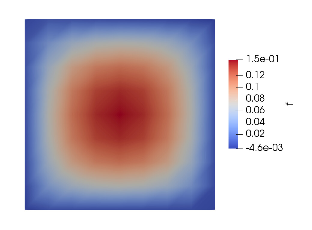
EDIT: With the above MWE, I obtain the following solution (without the discontinuity at x=0.5)

Thanks in advance for your help!

1 Like

Hi, making the following changes made the code work for me -

  1. Using from dolfinx import io instead of from dolfinx.io import XDMFFile
  2. Introducing a tol at interface like this -
tol = 1e-8
def marker_interface(x):
    return np.isclose(x[0], 0.5, tol)
  1. Replacing dot with inner like -
# diffusion
F += inner(grad(v), grad(u))*dx - inner(v*n, grad(u))*ds \
   - inner(avg(grad(v)), jump(u, n))*dS - inner(jump(v, n), avg(grad(u)))*dS \
   + gamma/avg(h)*inner(jump(v, n), jump(u, n))*dS

and

F += - inner(grad(v), u*n)*ds + alpha/h*v*u*ds\
   + uD*inner(grad(v), n)*ds - alpha/h*uD*v*ds
  1. Writing u to XDMFFile as -
with io.XDMFFile(MPI.COMM_WORLD, "uh.xdmf", "w") as file:
        file.write_mesh(u.function_space.mesh)
        file.write_function(u, 0)
        file.close()

Hence the whole code is -

from dolfinx import mesh, fem, nls, plot
from mpi4py import MPI
import ufl
from dolfinx import io
from petsc4py import PETSc
from ufl import dx, grad, dot, jump, avg
import numpy as np

msh = mesh.create_unit_square(MPI.COMM_WORLD, 8, 8)

V = fem.FunctionSpace(msh, ("DG", 1))

# create mesh tags
tol = 1e-8
def marker_interface(x):
    return np.isclose(x[0], 0.5, tol)

tdim = msh.topology.dim
fdim = tdim - 1
msh.topology.create_connectivity(fdim, tdim)
facet_imap = msh.topology.index_map(tdim - 1)
boundary_facets = mesh.exterior_facet_indices(msh.topology)
interface_facets = mesh.locate_entities(msh, tdim - 1, marker_interface)
num_facets = facet_imap.size_local + facet_imap.num_ghosts
indices = np.arange(0, num_facets)
values = np.zeros(indices.shape, dtype=np.intc)  # all facets are tagged with zero

values[boundary_facets] = 1
values[interface_facets] = 2

mesh_tags_facets = mesh.meshtags(msh, tdim - 1, indices, values) 

ds = ufl.Measure("ds", domain=msh, subdomain_data=mesh_tags_facets)
dS = ufl.Measure("dS", domain=msh, subdomain_data=mesh_tags_facets)

u = fem.Function(V)
u_n = fem.Function(V)
v = ufl.TestFunction(V)

h = ufl.CellDiameter(msh)
n = ufl.FacetNormal(msh)

# Define parameters
alpha = 10
gamma = 10

# Simulation constants
f = fem.Constant(msh, PETSc.ScalarType(2.0))

# Define variational problem
F = 0

# diffusion
F += inner(grad(v), grad(u))*dx - inner(v*n, grad(u))*ds \
   - inner(avg(grad(v)), jump(u, n))*dS - inner(jump(v, n), avg(grad(u)))*dS \
   + gamma/avg(h)*inner(jump(v, n), jump(u, n))*dS

# source
F += -v*f*dx 

# Dirichlet BC
uD = fem.Function(V)
uD.interpolate(lambda x: np.full(x[0].shape, 0.0))

F += - inner(grad(v), u*n)*ds + alpha/h*v*u*ds\
   + uD*inner(grad(v), n)*ds - alpha/h*uD*v*ds

problem = fem.petsc.NonlinearProblem(F, u)
solver = nls.petsc.NewtonSolver(MPI.COMM_WORLD, problem)
solver.solve(u)

with io.XDMFFile(MPI.COMM_WORLD, "uh.xdmf", "w") as file:
        file.write_mesh(u.function_space.mesh)
        file.write_function(u, 0)
        file.close()

Visualization in paraview -

Hi, this is not what I am looking for as it doesn’t satisfy the interface condition at x=0.5

I was able to get this far (a normal poisson problem) with the MWE provided.

So far I’ve manage to come up with this weak formulation that seems to be heading the right way.

F = 0

# diffusion
F += dot(grad(v), grad(u))*dx - dot(v*n, grad(u))*ds \
   - dot(avg(grad(v)), jump(u, n))*dS(0) - dot(jump(v, n), avg(grad(u)))*dS(0) \
   + gamma/avg(h)*dot(jump(v, n), jump(u, n))*dS(0)

# source
F += -v*f*dx 

# Dirichlet BC
F += - dot(grad(v), u*n)*ds + alpha/h*v*u*ds\
   + uD*dot(grad(v), n)*ds - alpha/h*uD*v*ds

K1 = fem.Constant(msh, PETSc.ScalarType(2.0))
K2 = fem.Constant(msh, PETSc.ScalarType(4.0))
F += u('-')/K1 * v('-') * dS(2) - u('+')/K2 * v('+') * dS(2)

However, this is still incorrect since when K1=K2 the field should be continuous and isn’t.

Have you tried approaching this from the primal or flux formulation? It might be easier to conceptualise the numerical fluxes over the interior facets you wish to constrain. At a glance it looks like you’re introducing a penalisation term but without a penalty parameter.

Not sure I get what you mean by the “primal or flux formulation”.

I’ve been trying to adapt this demo but I don’t understand how to get the Nitsche terms (symmetry and coercivity) for this specific interface condition.

unified analysis of DG paper Section 3 with careful choices of the fluxes \widehat{u} and \widehat{\sigma} on the interface.

Just a side comment on your physics, you gave your interface condition as

\frac{u(-)}{K(-)} = \frac{u(+)}{K(+)} \\ \nabla u(-) - \nabla u(+) = 0

This looks strange to me. “Normally” the scalar function would be continuous at the interface, and the discontinuity is in the field,

u(-) = u(+) \\ K(-)\nabla u(-) - K(+)\nabla u(+) = \sigma

At least that’s the case in electrostatics where u is the electrostatic potential, -K\nabla u is the electrostatic displacement vector (\mathbf{D}=\varepsilon \mathbf{E} = -\varepsilon\nabla u) and \sigma is the surface charge density along the interface. More precisely in that case the jump is in the perpendicular component,

\left(n(-), K(-)\nabla u(-)\right) + \left((n(+), K(+)\nabla u(+)\right) = \sigma

adjusting the sign in the jump to allow for the opposing directions of the two normal vectors.

1 Like

Such discontinuities occur for instance in the case of a thermal contact resistance (temperature jump) or conservation of chemical potential for mass transport (jump in concentration)

Fair enough. I must read more on the other uses of the Poisson equation :slight_smile:

Thanks for this.

I read through section 3 but I’m afraid my poor mathematical background is too light to understand a substantial fraction of this…

I’ll carry on looking for a demo :slight_smile:

This is the updated code for dolfinx 0.7.0

from dolfinx import mesh, fem, plot
import dolfinx.fem.petsc
import dolfinx.nls.petsc
from mpi4py import MPI
import ufl
from petsc4py import PETSc
from ufl import dx, grad, dot, jump, avg
import numpy as np

msh = mesh.create_unit_square(MPI.COMM_WORLD, 8, 8)

V = fem.FunctionSpace(msh, ("DG", 1))
uD = fem.Function(V)
uD.interpolate(lambda x: np.full(x[0].shape, 0.0))

# create mesh tags
def marker_interface(x):
    return np.isclose(x[0], 0.5)

tdim = msh.topology.dim
fdim = tdim - 1
msh.topology.create_connectivity(fdim, tdim)
facet_imap = msh.topology.index_map(tdim - 1)
boundary_facets = mesh.exterior_facet_indices(msh.topology)
interface_facets = mesh.locate_entities(msh, tdim - 1, marker_interface)
num_facets = facet_imap.size_local + facet_imap.num_ghosts
indices = np.arange(0, num_facets)
# values = np.arange(0, num_facets, dtype=np.intc)
values = np.zeros(indices.shape, dtype=np.intc)  # all facets are tagged with zero

values[boundary_facets] = 1
values[interface_facets] = 2

mesh_tags_facets = mesh.meshtags(msh, tdim - 1, indices, values) 

ds = ufl.Measure("ds", domain=msh, subdomain_data=mesh_tags_facets)
dS = ufl.Measure("dS", domain=msh, subdomain_data=mesh_tags_facets)

u = fem.Function(V)
u_n = fem.Function(V)
v = ufl.TestFunction(V)

h = ufl.CellDiameter(msh)
n = ufl.FacetNormal(msh)

# Define parameters
alpha = 10
gamma = 10

# Simulation constants
f = fem.Constant(msh, PETSc.ScalarType(2.0))

# Define variational problem

F = 0

# diffusion
F += dot(grad(v), grad(u))*dx - dot(v*n, grad(u))*ds \
   - dot(avg(grad(v)), jump(u, n))*dS(0) - dot(jump(v, n), avg(grad(u)))*dS(0) \
   + gamma/avg(h)*dot(jump(v, n), jump(u, n))*dS(0)

# source
F += -v*f*dx 

# Dirichlet BC
F += - dot(grad(v), u*n)*ds + alpha/h*v*u*ds\
   + uD*dot(grad(v), n)*ds - alpha/h*uD*v*ds

K1 = fem.Constant(msh, PETSc.ScalarType(2.0))
K2 = fem.Constant(msh, PETSc.ScalarType(4.0))
F += u('-')/K1 * v('-') * dS(2) - u('+')/K2 * v('+') * dS(2)

# symmetry
F += - dot(avg(grad(v)), jump(u/K1, n))*dS(2)
F += - dot(avg(grad(v)), jump(u/K2, n))*dS(2)
# coercivity
F += + gamma/avg(h)*dot(jump(v, n), jump(u/K1, n))*dS(2)
F += + gamma/avg(h)*dot(jump(v, n), jump(u/K2, n))*dS(2)

problem = dolfinx.fem.petsc.NonlinearProblem(F, u)
solver = dolfinx.nls.petsc.NewtonSolver(MPI.COMM_WORLD, problem)
solver.solve(u)

import pyvista
pyvista.OFF_SCREEN = True

pyvista.start_xvfb()

u_topology, u_cell_types, u_geometry = plot.vtk_mesh(V)
u_grid = pyvista.UnstructuredGrid(u_topology, u_cell_types, u_geometry)
u_grid.point_data["u"] = u.x.array.real
u_grid.set_active_scalars("u")
u_plotter = pyvista.Plotter()
u_plotter.add_mesh(u_grid, show_edges=False)
u_plotter.view_xy()
if not pyvista.OFF_SCREEN:
    u_plotter.show()
else:
    figure = u_plotter.screenshot("DG.png")

Does it work exactly as intended? I’m asking because I’m still very interested in this (I am the asker in your link of your 1st post), and I got stuck.

It’s not working at the minute and I must admit we are all banging our head against the wall with this because the maths aren’t trivial and we are not maths people :joy:

I see… This shouldn’t be rocket science. Physically, it is very simple, there’s a discontinuity in the voltage or temperature (a scalar field), that is proportional to a resistance (electrical or thermal in those 2 cases). Extremely simple mathematically.
This is implemented in COMSOL and in a myriad of other FEM solvers. There’s no reason this should involve recent papers for FEniCSx, IMO. Unless one wants to use a strange and/or very complicated way to accomplish what should be easy.

I am also interested in how to code this in dolfinx. In my problem, I have a discontinuity in the field at the internal boundary with the flux proportional to the jump in the field:

\nabla u \cdot \hat{\mathbf{n}} = \alpha (u_{+} - u_{-}) where \alpha \in \mathbb{R}

I also used the DG formulation with the appropriate penalty terms but I cannot get the discontinuity condition right.
As @raboynics has pointed out, this is already done in COMSOL, so I assumed it would not be unreasonably complicated in FEniCSx.

1 Like

Isn’t there a jump missing in the boundary condition here? What side is the

Evaluated at?
This is a discontinuous quantity, and the normal is pointing in different directions depending on what cell you are in.

I have
\nabla u \cdot \hat{n}(+) = \alpha (u_{+} - u_{-})
and because the flux is continuous, then I also have
\nabla u \cdot \hat{n}(-) = \alpha (u_{-} - u_{+})

This seems to do the job, the jump at the interface is equal to 0.5 as expected from setting K1 = 2 and K2 = 4.

Basically, I worked out the jump term in the integral at the interface according to the interface condition.

\frac{u(-)}{K(-)} = \frac{u(+)}{K(+)}
||u|| = u(+) - u(-) = u(-)\left(\frac{K1}{K2}-1\right)

The same approach works also for the interface condition:

\frac{u(-)}{K(-)}= \frac{u(+)^2}{K(+)^2}

from dolfinx import mesh, fem, plot, geometry
import dolfinx.fem.petsc
import dolfinx.nls.petsc
from mpi4py import MPI
import ufl
from petsc4py import PETSc
from ufl import dx, grad, dot, jump, avg
import numpy as np
import matplotlib.pyplot as plt
import pyvista


msh = mesh.create_unit_square(MPI.COMM_WORLD, 100, 100)
V = fem.FunctionSpace(msh, ("DG", 1))
uD = fem.Function(V)
uD.interpolate(lambda x: np.full(x[0].shape, 0.0))

# create mesh tags
def marker_interface(x):
    return np.isclose(x[0], 0.5)

tdim = msh.topology.dim
fdim = tdim - 1
msh.topology.create_connectivity(fdim, tdim)
facet_imap = msh.topology.index_map(tdim - 1)
boundary_facets = mesh.exterior_facet_indices(msh.topology)
interface_facets = mesh.locate_entities(msh, tdim - 1, marker_interface)
num_facets = facet_imap.size_local + facet_imap.num_ghosts
indices = np.arange(0, num_facets)
# values = np.arange(0, num_facets, dtype=np.intc)
values = np.zeros(indices.shape, dtype=np.intc)  # all facets are tagged with zero

values[boundary_facets] = 1
values[interface_facets] = 2

mesh_tags_facets = mesh.meshtags(msh, tdim - 1, indices, values) 

ds = ufl.Measure("ds", domain=msh, subdomain_data=mesh_tags_facets)
dS = ufl.Measure("dS", domain=msh, subdomain_data=mesh_tags_facets)
u = fem.Function(V)
u_n = fem.Function(V)
v = ufl.TestFunction(V)

h = ufl.CellDiameter(msh)
n = ufl.FacetNormal(msh)

# Define parameters
alpha = 1000

# Simulation constants
f = fem.Constant(msh, PETSc.ScalarType(2.0))
K1 = fem.Constant(msh, PETSc.ScalarType(2.0))
K2 = fem.Constant(msh, PETSc.ScalarType(4.0))

# Define variational problem
F = 0
F += dot(grad(v), grad(u))*dx - dot(v*n, grad(u))*ds \
   - dot(avg(grad(v)), jump(u, n))*dS(0) - dot(jump(v, n), avg(grad(u)))*dS(0) \
   + alpha/avg(h)*dot(jump(v, n), jump(u, n))*dS(0) + alpha/h*v*u*ds

# source
F += -v*f*dx 

# Dirichlet BC
F += - dot(grad(v), u*n)*ds \
   + uD*dot(grad(v), n)*ds - alpha/h*uD*v*ds

# Interface 
F += - dot(avg(grad(v)), n('-'))*(u('-')*(K1/K2-1))*dS(2)
F += alpha/avg(h)*dot(jump(v,n),n('-'))*(u('-')*(K1/K2-1))*dS(2)

# symmetry
F += - dot(avg(grad(v)), jump(u, n))*dS(2)
# coercivity
F += + alpha/avg(h)*dot(jump(v, n), jump(u, n))*dS(2)

problem = dolfinx.fem.petsc.NonlinearProblem(F, u)
solver = dolfinx.nls.petsc.NewtonSolver(MPI.COMM_WORLD, problem)
solver.solve(u)

bb_tree = geometry.bb_tree(msh, msh.topology.dim)
n_points = 1000
tol = 0.001  # Avoid hitting the outside of the domain
x = np.linspace(0 + tol, 1 - tol, n_points)
y = np.ones(n_points)*0.5
points = np.zeros((3, n_points))
points[0] = x
points[1] = y
u_values = []
cells = []
points_on_proc = []
# Find cells whose bounding-box collide with the the points
cell_candidates = geometry.compute_collisions_points(bb_tree, points.T)
# Choose one of the cells that contains the point
colliding_cells = geometry.compute_colliding_cells(msh, cell_candidates, points.T)
for i, point in enumerate(points.T):
    if len(colliding_cells.links(i)) > 0:
        points_on_proc.append(point)
        cells.append(colliding_cells.links(i)[0])
points_on_proc = np.array(points_on_proc, dtype=np.float64)
u_values = u.eval(points_on_proc, cells)
fig = plt.figure()
plt.plot(points_on_proc[:, 0], u_values, "k", linewidth=2)
plt.grid(True)
plt.show()

pyvista.OFF_SCREEN = True

pyvista.start_xvfb()

u_topology, u_cell_types, u_geometry = plot.vtk_mesh(V)
u_grid = pyvista.UnstructuredGrid(u_topology, u_cell_types, u_geometry)
u_grid.point_data["u"] = u.x.array.real
u_grid.set_active_scalars("u")
u_plotter = pyvista.Plotter()
u_plotter.add_mesh(u_grid, show_edges=False)
u_plotter.view_xy()
if not pyvista.OFF_SCREEN:
    u_plotter.show()
else:
    figure = u_plotter.screenshot("DG.png")

immagine

4 Likes

Hey, I am facing the same issue so I tried to run this code updated with import modifications without which it is not working for me

Here is the updated code

import dolfinx.nls.petsc
from dolfinx import mesh, fem, nls, plot
from mpi4py import MPI
import ufl
from dolfinx import io
from petsc4py import PETSc
from ufl import dx, grad, dot, jump, avg, inner

from dolfinx.fem.petsc import (LinearProblem, assemble_matrix, create_vector, assemble_vector, 
                                apply_lifting, set_bc, NonlinearProblem )

import numpy as np

msh = mesh.create_unit_square(MPI.COMM_WORLD, 8, 8)

V = fem.FunctionSpace(msh, ("DG", 1))

# create mesh tags
tol = 1e-8
def marker_interface(x):
    return np.isclose(x[0], 0.5, tol)

tdim = msh.topology.dim
fdim = tdim - 1
msh.topology.create_connectivity(fdim, tdim)
facet_imap = msh.topology.index_map(tdim - 1)
boundary_facets = mesh.exterior_facet_indices(msh.topology)
interface_facets = mesh.locate_entities(msh, tdim - 1, marker_interface)
num_facets = facet_imap.size_local + facet_imap.num_ghosts
indices = np.arange(0, num_facets)
values = np.zeros(indices.shape, dtype=np.intc)  # all facets are tagged with zero

values[boundary_facets] = 1
values[interface_facets] = 2

mesh_tags_facets = mesh.meshtags(msh, tdim - 1, indices, values) 

ds = ufl.Measure("ds", domain=msh, subdomain_data=mesh_tags_facets)
dS = ufl.Measure("dS", domain=msh, subdomain_data=mesh_tags_facets)

u = fem.Function(V)
u_n = fem.Function(V)
v = ufl.TestFunction(V)

h = ufl.CellDiameter(msh)
n = ufl.FacetNormal(msh)

# Define parameters
alpha = 10
gamma = 10

# Simulation constants
f = fem.Constant(msh, PETSc.ScalarType(2.0))

# Define variational problem
F = 0

# diffusion
F += inner(grad(v), grad(u))*dx - inner(v*n, grad(u))*ds \
   - inner(avg(grad(v)), jump(u, n))*dS - inner(jump(v, n), avg(grad(u)))*dS \
   + gamma/avg(h)*inner(jump(v, n), jump(u, n))*dS

# source
F += -v*f*dx 

# Dirichlet BC
uD = fem.Function(V)
uD.interpolate(lambda x: np.full(x[0].shape, 0.0))

F += - inner(grad(v), u*n)*ds + alpha/h*v*u*ds\
   + uD*inner(grad(v), n)*ds - alpha/h*uD*v*ds

problem = NonlinearProblem(F, u)
solver = nls.petsc.NewtonSolver(MPI.COMM_WORLD, problem)
solver.solve(u)

with io.XDMFFile(MPI.COMM_WORLD, "uh.xdmf", "w") as file:
        file.write_mesh(u.function_space.mesh)
        file.write_function(u)
        file.close()

But I get the following error

Traceback (most recent call last):
  File "/mnt/c/Users/quent/Documents/Codes/FENICSX/Examples/Jump/FromDiscourse/Discontinuity.py", line 85, in <module>
    file.write_function(u)
  File "/home/quentin_digimind/anaconda3/envs/fenicsx-env/lib/python3.12/site-packages/dolfinx/io/utils.py", line 235, in write_function
    super().write_function(getattr(u, "_cpp_object", u), t, mesh_xpath)
RuntimeError: Function and Mesh dof layouts do not match. Maybe the Function needs to be interpolated?

Any idea about How I can correct this ?

Thanks,

Quentin